Integrating the No-Code Quant Backtester into the Russian Doll Engine

We started off with the conceptualisation of trading alpha in different abstract representations, such as mathematical formulas, graphs and visual representations:

Alpha-Encoding Data Structures

For machine trading this would require a convenient translation between the different representations onto computer bits, and we implemented those data structures and algorithms:

Programmatic Quant Alpha Encoding with Python

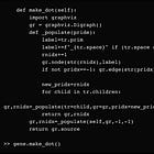
In order to make use of these data structures, we would require very specific graph traversal algorithms determining the order of evaluation. In addition, recursive thinking was employed to truly appreciate our modelling of the problem:

Traversal Algorithms for Alpha Tree/Graph and Recursion Exercises

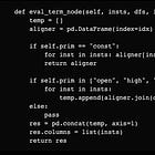
In particular, each alpha graph is thought to be composed of sub-alphas, at least in the modelling sense, even if there were no semantic sense for this path of thinking. We then created a no-code quantitative backtesting engine using these building blocks by defining code logic for predetermined primitive structures:

Building a No Code Quantitative Backtest Engine for Machine Trading (with Python)

The update to the Russian Doll engine was last given here:

Integration of the Quadratic Optimizer into the Python Backtester (Code Dump of the updated Russian Doll Engine)

In this post we demonstrate how to integrate the Russian Doll module to our automatic evaluation module. Refer to the Russian Doll module code in that post, no change has been made.

The survey we conducted from readers show that only about half of the current consumers of our content are able to keep pace with the current advanced programming lecture series; from the next week onwards, we are going to start from the very basics and code our way up to what we have on our hands today, reviewing many of the technical details. We will also document this on to the market notes. This will be a fantastic review for advanced programmers, and supplementary material for the new readers.

For this post, we are going to assume you know how to use the Alpha module object from our Russian Doll package, and go right into the programming part. If you don’t, you can download the code and survey our code, but I assume that will require a fair bit of technical depth. So if you aren’t there yet, bare with me and hop on the journey next week.

As in last post, say we already got the SP500 OHLCV data:

async def main():    
    formula="csrank(neg(minus(const_1,div(open,close))))" 
    #Alpha#33: rank((-1 * ((1 - (open / close))^1))) 
    #https://arxiv.org/pdf/1601.00991.pdf
    
    res = requests.get("https://en.wikipedia.org/wiki/List_of_S%26P_500_companies")
    soup = BeautifulSoup(res.content,'lxml')
    table = soup.find_all('table')[0] 
    df = pd.read_html(str(table))       
    tickers=list(df[0].Symbol)
    
    dfs={}

    def poll(ticker):
        dobj=yf.Ticker(ticker)
        dhist=dobj\
            .history(start="2000-01-01")\
            .reset_index()
        if dhist is None or dhist.empty:
            return
        dhist=dhist.rename(
            columns={
                "Date": "datetime",
                "Open": "open",
                "High": "high",
                "Low": "low",
                "Close": "close",
                "Volume": "volume",
            })\
            .drop(columns=["Dividends","Stock Splits"])   
        dhist["datetime"]=dhist["datetime"].dt.tz_localize(pytz.utc)
        dfs[ticker]=dhist.reset_index(drop=True).set_index("datetime")
    
    threads=[]  
    for ticker in tickers:
        threads.append(threading.Thread(target=poll, args=(ticker,)))
    for thread in threads:
        thread.start()
    for thread in threads:
        thread.join()
  
    insts=list(dfs.keys())
    dfs={inst:dfs[inst] for inst in insts}
    start_idx=min([list(df.index)[0] for df in dfs.values()])
    end_idx=max([list(df.index)[-1] for df in dfs.values()])

We want to have a very simple interface, say:

    gene=Gene.str_to_gene(formula)
    strat = GeneticAlpha(
        genome=gene, 
        trade_range=(start_idx,end_idx), 
        instruments=insts, 
        dfs=dfs
    )
    df=await strat.run_simulation(verbose=False)
    import matplotlib.pyplot as plt
    plt.plot(np.log(df.capital))
    plt.show()

where for those familiar, the run_simulation method comes from our BaseAlpha class in the Russian Doll library. That means the GeneticAlpha module extends the Alpha module (which extends the BaseAlpha module). The logic code in run_simulation to perform the pnl computation and backtesting is all handled by the Russian Doll, so we are not doing anything new here. We just have to link the signal generation component, which we already implemented in the last post, to the signal generation method that has to be implemented by any parent instance of the Alpha class in the compute_forecasts function.

For those already familiar, we will do this in the compute_signals_unaligned function, and we write:

class GeneticAlpha(Alpha):
    def __init__(
        self,
        genome,
        trade_range=None,
        instruments=[], 
        execrates=None,
        commrates=None,
        longswps=None,
        shortswps=None, 
        dfs={},  
        positional_inertia=0,
        specs={"quantile":((0.00,0.10),(0.90,1.00),)},
        use_cache=False
    ):
        if not use_cache: genome=Gene.str_to_gene(str(genome))
        super().__init__(
            trade_range=trade_range, 
            instruments=instruments, 
            execrates=execrates,
            commrates=commrates,
            longswps=longswps,
            shortswps=shortswps,
            dfs=dfs,
            positional_inertia=positional_inertia 
        )
        self.genome = genome
        self.specs=specs

     ..................

    async def compute_signals_unaligned(self, shattered=True, param_idx=0, index=None):
        alphadf = self.genome.evaluate_node(insts=self.instruments, dfs=self.dfs, idx=index)
        self.pad_ffill_dfs["alphadf"] = alphadf
        return
    
    async def compute_signals_aligned(self, shattered=True, param_idx=0, index=None):
        return 

where we already implemented the evaluate_node method in the previous post. The quantiles say we want to go l/s the top and bottom deciles.

The rest would be just instantiating the variables to create the forecasting dataframe:

    def instantiate_eligibilities_and_strat_variables(self, delta_lag=0):
        self.alphadf = self.pad_ffill_dfs["alphadf"]
        eligibles = []
        for inst in self.instruments:
            inst_eligible = (~pd.isna(self.alphadf[inst])) \
                & self.activedf[inst].astype("bool") \
                & (self.voldf[inst] > 0.00001).astype("bool") \
                & (self.baseclosedf[inst] > 0).astype("bool") \
                & (self.retdf[inst].shift(-1) < 0.30).astype("bool") #dirty handling of unclean data
            eligibles.append(inst_eligible)
        
        self.invriskdf = np.log(1 / self.voldf) / np.log(1.3)
        self.eligiblesdf = pd.concat(eligibles, axis=1)
        self.eligiblesdf.columns = self.instruments
        self.eligiblesdf.astype("int8")       
        rankdf = (self.alphadf.div(self.eligiblesdf, axis=1)).replace([np.inf, -np.inf], np.nan).rank(
            axis=1, method="first", na_option="keep", ascending=True
        )
        trade_quantiles=self.specs["quantile"]
        candidates_ranked = len(self.instruments) - rankdf.isnull().sum(axis=1)
        nl=trade_quantiles[1][1]-trade_quantiles[1][0]
        ns=trade_quantiles[0][1]-trade_quantiles[0][0]
        nl=np.ceil(nl*candidates_ranked)
        ns=np.ceil(ns*candidates_ranked)
        long_cutoffs=(np.floor(trade_quantiles[1][0]*candidates_ranked),np.floor(trade_quantiles[1][0]*candidates_ranked)+nl)
        short_cutoffs=(np.ceil(trade_quantiles[0][1]*candidates_ranked),np.ceil(trade_quantiles[0][1]*candidates_ranked)-ns)

        long_df = np.logical_and(rankdf.gt(long_cutoffs[0], axis=0), rankdf.le(long_cutoffs[1], axis=0)).astype("int32")
        short_df = np.logical_and(rankdf.le(short_cutoffs[0], axis=0), rankdf.gt(short_cutoffs[1], axis=0)).astype("int32")
        forecast_df = long_df - short_df
        self.forecast_df = forecast_df
        return

    def compute_forecasts(self, portfolio_i, date, eligibles_row):
        return self.forecast_df.loc[date], np.sum(eligibles_row)

This will definitely be difficult for unfamiliar readers, so readers (paid) should just download the appended code at the bottom of the post:

Again, if you are not used to reading source code, this would be too overwhelming for you, and over the next few months, we are going to from writing a simple, unoptimised single strategy Python tester, to multi strategy testers, to optimised and vector testing scripts, to the Russian Doll and ultimately the no-code programmatic evaluation tool that we have demonstrated today. So…jump on board if you haven’t already, and be prepared to get your hands dirty with programming (no, chatgpt will not save you here).

Code: (paid)