Traversal Algorithms for Alpha Tree/Graph and Recursion Exercises
In the last quant dev post:
we implemented the alpha tree, which extended from our discussion on abstract mathematical representations to computer bits for machine trading.
So we have a data structure, which in general, serve dual purposes: rule-based information storage and efficient/systematic access. There are many data structures; lists, arrays, sets, tuples, dictionaries, heaps, trees, stack, graphs, you name it.
In our particular case, the tree structure was most apropos, and since the objects themselves may not be memory efficient or readable, our translation between their formulaic and object representations proved useful.
But we will primarily be working with this data structure encoding in the programmatic sense, which means we need to be comfortable with traversing the nodes in the graph.
Fortunately, if one is familiar with recursive thinking, this would not be a demanding task. It is synonymous with how one would do mathematical induction, for instance, in the construction of a proof.
This post is a gentle introduction to recursion, and also implements the specific algorithms required for our alpha graph. When we write more recursion algorithms in future posts, it will be assumed all readers are sufficiently familiar.
Recursion is just something that repeats. For instance, LINUX Is Not UniX is a recursive acronym, because the phrase acronyms to LINUX, which expanded, acronyms again to LINUX and so on. So, how does that occur in programming?
Suppose we were to take integer powers. a^b = a * a**(b-1). Well that’s particularly obvious. A recursion consists of the base case, and the recursive case (the sub-problem).
def power(a,b):
    if b==0:
        return 1
    if b==1:
        return a
    return a*power(a,b-1)
Well that’s easy. Another one:
def factorial(n):
    if n == 0 or n == 1:
        return 1
    else:
        return n*factorial(n-1)
But also maybe there are more than one sub-problem, like in the Fibonacci sequence:
def fibonacci(n):
    if n < 0:
        raise Exception()
    if n == 1 or n == 2:
        return 1
    else:
        return fibonacci(n - 1) + fibonacci(n - 2)
or maybe we have a recursive algorithm on a data structure, to sum a list of numbers:
def sum_list(lst):
    if len(lst) == 0:
        return 0
    if len(lst) == 1:
        return lst[0]
    else:
        return lst[0] + sum_list(lst[1:])
So well these are pretty trivial examples, but you get the idea. You just encode the solution to ‘the most atomic problem’, and make a recursive call to sub-problems. Okay, just one more example that is perhaps more complicated to see if you catch on, all permutations:
def generate_permutations(array):
    if len(array) <= 1:
        return [array]
    permutations = []
    for i in range(len(array)):
        element = array[i]
        sub_sequence = array[:i] + array[i+1:]
        sub_permutations = generate_permutations(sub_sequence)
        for permutation in sub_permutations:
            permutations.append([element]+permutation)
    assert len(permutations) == factorial(len(array))
    return permutations
Basically, the algorithm says, the singleton permutation is itself, and otherwise append each letter to the head of (well, it could be anywhere really) every other subsequence permutation. Anyway, there are more things to know, in practice, like algorithmic complexity. * This leads to techniques such as memoization and dynamic programming.
*Consider the fibonacci example. fib(5) would call fib(4),fib(3), and fib(4) would call fib(3),fib(2)…so we have called fib(3) minimally twice. We are wasting compute, and if you consider the call stack, you make \ord(2^n) calls, although you could easily compute this in linear time. Actually, assuming a constant time arithmetic model, its \ord(1).
But we digress. In the future, we would study design and analysis of algorithms in our market notes, but let’s move on for now. Of particular importance in the consideration of alpha models in machine trading is model complexity. In general, Occam’s razor applies to market phenomena - complexity is not favoured. Although the formula might be used in determining semantic complexity in the discretionary sense, the number of nodes, height of the alpha tree give insights into the syntactic complexity. We can employ recursion.
'''
Defines a formulaic quant rule

prim
space: identifies a primitive from its primitive space

children = *[]
parent
is_terminal
size()
height()
depth()
'''
import numpy as np
class Gene():

    @staticmethod
    def str_to_gene(strgene):
        #refer to previous

    def __init__(self, prim, space, \
        is_terminal, parent=None, children=None
    ):
        #refer to previous

    def size(self):
        if not self.children:
            return 1
        return 1 + np.sum([child.size() for child in self.children])

    def depth(self):
        if not self.parent:
            return 0
        return 1 +  self.parent.depth()

    def height(self):
        if len(self.children) == 0:
            return 0
        return 1 + np.max([child.height() for child in self.children])

    def __repr__(self):
        if self.is_terminal:
            res=self.prim
            res+=f"_{self.space}" if (self.space or self.space == 0) else ""
            return res
        res=f"{self.prim}"
        res+=f"_{self.space}" if (self.space or self.space == 0) else ""
        args=[]

        for child in self.children:
            args.append(str(child))
        return res + "(" + ",".join(args) + ")"
And these work:
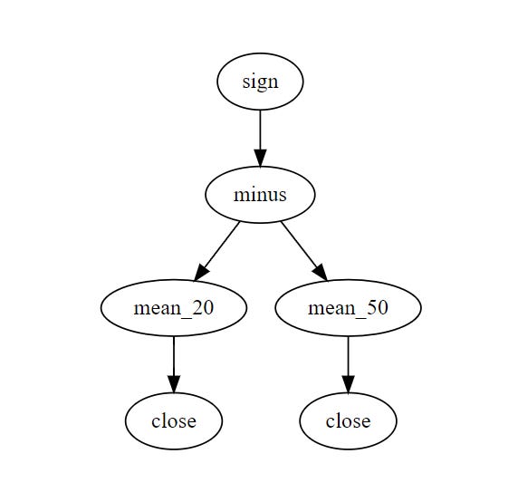
    formula="sign(minus(mean_20(close),mean_50(close)))"
    gene=Gene.str_to_gene(formula)
    print(gene)
    print(formula)
    print(gene.height()) #3
    print(gene.depth()) #0
    print(gene.size()) #6
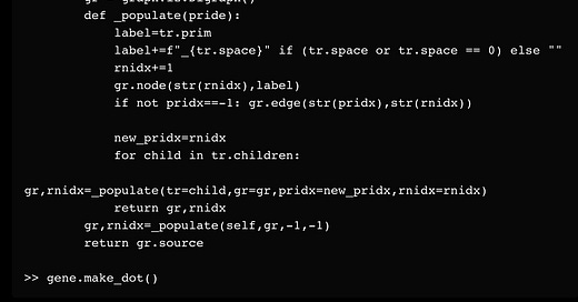
Any say we want to use the DOT language to create a visual representation of this alpha data structure, we can use the graphviz package and instantiate a directed graph using recursion:
    def make_dot(self):
        import graphviz
        gr = graphviz.Digraph()
        def _populate(pride):
            label=tr.prim
            label+=f"_{tr.space}" if (tr.space or tr.space == 0) else ""
            rnidx+=1
            gr.node(str(rnidx),label)
            if not pridx==-1: gr.edge(str(pridx),str(rnidx))

            new_pridx=rnidx
            for child in tr.children:
                gr,rnidx=_populate(tr=child,gr=gr,pridx=new_pridx,rnidx=rnidx)
            return gr,rnidx
        gr,rnidx=_populate(self,gr,-1,-1)
        return gr.source

>> gene.make_dot()
and then copy paste this string into https://dreampuf.github.io/GraphvizOnline/
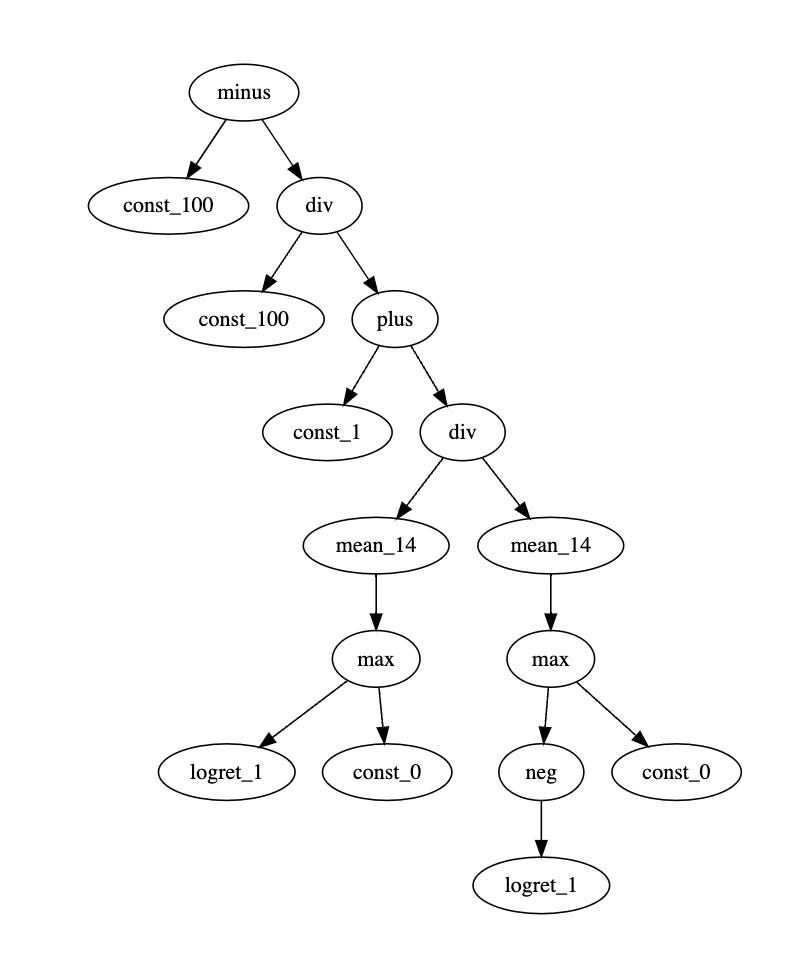
Well this is trivial, perhaps, but then maybe you try decoding something like this:
minus(const_100,div(const_100,plus(const_1,div(mean_14(max(logret_1(),const_0)),mean_14(max(neg(logret_1()),const_0))))))
and you won’t have a fun time…but this actually turns out to be the computation of a 14-day RSI.
Anyway, we are almost done. We just wanted to talk about traversals and orders of evaluation, and see 3 algorithms. Maybe this one will hurt your brain slightly more. Basically the point we want to bring across is that the order of evaluations matter.
Assume you have an alpha graph, in what order would you explore the nodes? For simplicity, let’s assume balanced, full binary tree.
Pre-order traversal: visit yourself then your children.
formula="1(2(3,4),5(6,7))"
gene=Gene.str_to_gene(formula)
print(gene.make_dot())
To trace how the algorithm traverses, you can put a dot on the left of each node, and then try to trace (starting from the left) without lifting up your pen while hugging the graph. Simple trick. If you trace the graph like this and print the node every time our tracing hits the blue dot, we get 1-7 ordered. But we can do other traversals:
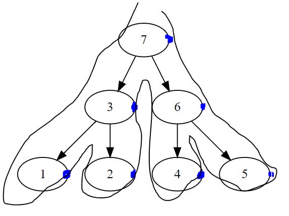
Post-order traversal: visit your children then yourself.
formula="7(3(1,2),6(4,5))"
gene=Gene.str_to_gene(formula)
print(gene.make_dot())
Again, you trace the graph but with the dot on the right hand side of the node. The graph itself is different, but again you get 1-7 ordered. Okay one more, (note while post-pre order traversals are general tree traversals, the next one only applies to binary trees):
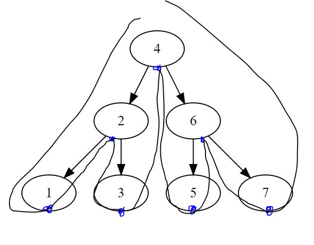
In-order traversal: visit left, check yourself, visit right.
formula="4(2(1,3),6(5,7))"
gene=Gene.str_to_gene(formula)
print(gene.make_dot())
Again a different graph, dot the middle of the node, and trace. You get 1-7 ordered. So…traversal order matters.
So what do we need?
I don’t know about you but I’d pick post-order traversal…see the sub-rule:
minus(mean_20(close),mean_50(close))to compute the minus, you would already to have evaluated both the rolling average in the 20/50 period, which are the children nodes. So you would have visited them, and gotten them to give us the computation results before we invoke the subtraction node.
Actually we already did pre-order traversals, although maybe in a non-obvious way. See:
    def height(self):
        if len(self.children) == 0:
            return 0
        return 1 + np.max([child.height() for child in self.children])
but the post-order variant would be
    def height(self):
        if len(self.children) == 0:
            return 0
        return np.max([child.height() for child in self.children]) + 1
which in this case doesn’t really matter since we are maintaining the state within the call stack inside the return values. Just thought I’d mention.
Cool, now you know recursion.
Moving forward, we would like to use recursion to write a host of other useful algorithms, such as the generation of trees, evaluation…and so on.
Bringing it all together, here is the current state of all our code on our running advanced quant dev series, from formulaic representations, machine encoding/decoding and recursion algorithms:
Code File (paid):

