In the previous lecture, we did a line by line walk through and intuitive explanation of the need for volatility targeting:
In particular, the expectation for risk-adjusted returns shall be commensurate with our position sizing. The risk-adjustment is made by taking position sizes inversely proportional to their price volatility, and the overall leverage is matched dynamically to hit a desired portfolio volatility level.
The alpha instance was a trend-following strategy, where the alpha forecast was 1 when fast MA > slow MA and 0 otherwise, indicating a positive, long position when the asset price is trending up and a flat (no) position otherwise.
Since the alpha forecast is binary-ily zero or one, we said that there is only the ability to indicate the presence, but not the degree of trend-iness in asset prices. As a result, there is not much flexibility in our ability to encode for EV preference, since for all the trending markets, our EV is uniformly one.
In this post, we want to address two common problem groups identified in the beginner quant - the first is…well we want to be able to encode our ‘EV’ expectation in a more granular fashion, indicating our degree of `want to trade’. Well you might think that if your alpha forecast is continuous to begin with, then you won’t have such a problem. What do I mean?
Imagine your strategy is to buy `oversold’ stocks, and your methodology is purchasing when 14-Day RSI < 20 score. So your forecast is perhaps something like
1 if (20 - RSI(14) > 0) else 0.
But you want a continuous signal, and since RSI is continuous, then to indicate the degree of `oversold’ness, you might encode your alpha forecast as follows:
max(20 - RSI(14), 0)
so when RSI(14) > 20, it is not considered oversold, and you are flat, otherwise you increase your position relative to how much lower it is to twenty. Well that is perhaps a reasonable line of thinking, and I would not argue about whether it is astute or not. You certainly would have managed to go from a digital to an analog signal, and your position sizing is more nuanced and varied. Here is the second problem group I want to target - why 14-day? Why 20 cutoff?
This second group believes in the holy grail of optimization. I call this the YouTube Finance crowd. Go to Youtube, search best “moving average crossover strategy”, “best RSI strategy”…and they always have some nice parameters prepared for you. Then they plot it on their candlestick charts, zoom in on two or three occasions where the parameters worked a beauty and convince you to that trading capital is easy.
First, let’s consider the improbability of this statement. Say you want to choose moving average pair parameters. You decide that any moving average window between 5-200 is reasonable. That is 196 numbers. How many pairs can you come up with? 196 choose 2 = 19110. Your favourite YouTube technical trader aficionado suggested one. And his pair is the best? Assuming any pair is likely to be as good as the other….his suggestion is likely to be indeed the best pair with 0.00005 probability. Also, that is assuming there is a best pair. Well, historically speaking, the best pair exists, because…history is static. Static optimization has an optimum, but you don’t trade markets in the past. You trade the future…right? And markets move, so do optimums. In a dynamically moving global optima…your chances of choosing the best moving average crossover pair? Infinitesimal.
Sure, I am not saying optimization is bad…in machine learning algorithms and many nuanced applications, fine tuning and parameter optimization is key to obtaining convergence and optimal solutions. I am just saying, your technical indicator rule based strategy? I say it not be so.
I am saying we should not optimise much, or even at all in most scenarios. I am not saying I know the best parameter, I am saying nobody does, and we should just take signals from a variety of parameters. We can treat each parameter set as sub-strategy in itself, which has some forecast, and then take the combination of these forecasts from different parameter sets…as if we are collecting votes.
One immediate benefit is that we solve the problem of having too little bits encode our EV for the position. Instead of having just zero or one forecast….since we are taking binary votes from multiple subsystems, our signal forecast becomes more continuous - naturally our degree of `want to trade’ is encoded in the relative magnitude of combined forecasts.
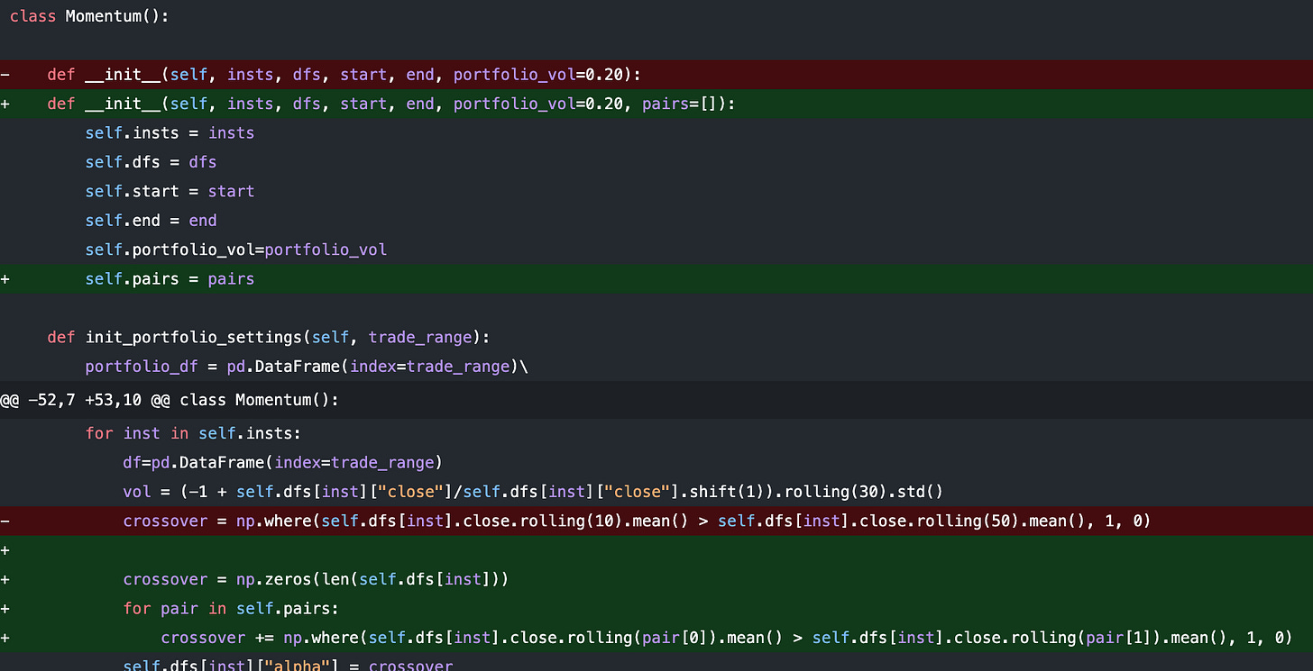
It may just be easier to show you. Consider the trend following strategy, from the previous code…again we make minimal changes. The code is attached below for paid readers, but you should be able to follow along either way. We highlight the adjustments, so be sure to read the previous post.
Instead of hard-encoding the moving average pair, we let our Momentum object take in a MA-pair parameter:
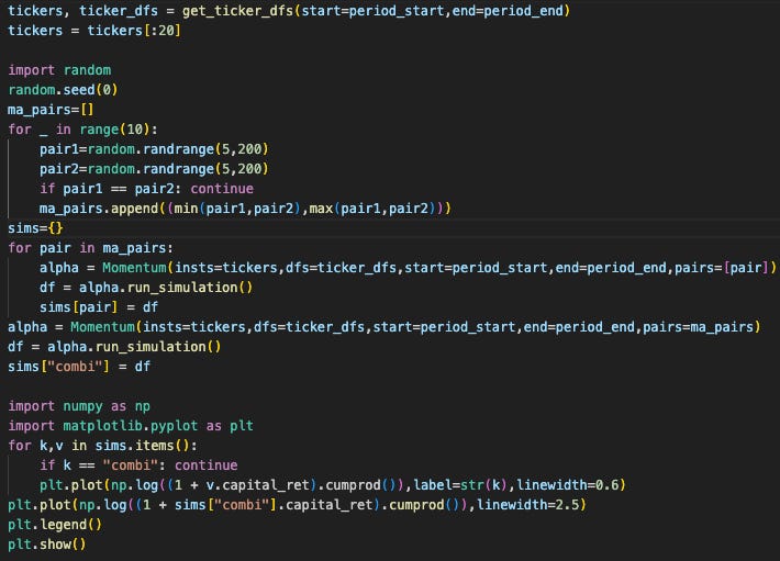
Inside the main.py file, we now generate 10 different MA average pairs, which correspond to 10 different MA crossover strategies. We create a 11-th one, which is the combined MA crossover taking votes from all the 10 different crossovers.
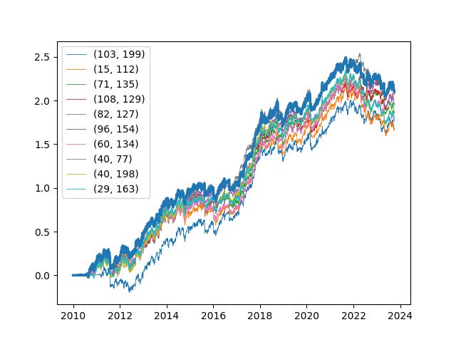
Let’s take a look at the PnL, with the combined in thick blue:
The 10 different crossover pairs each had their moments to shine…in some periods, one crossover performed better than the other. However, it is clear that over the entirety of the backtest, the combined strategy was the most consistent performer.
We only took a small sample size of 20 tickers, but it is likely that this outperformance would be even more distinct once we increase our sample size. Intuitively, we are sizing up when the degree of trend is more significant. On one hand, our degree of EV specification is more nuanced, albeit imperfect. On the other, these sub-forecasts have imperfect correlations, which represent diversifying benefits.
I’m sure you would have heard - diversify, diversify, diversify. But it is not just an old adage based on common sense about prudent wealth management. It is underpinned by the mathematics of portfolio management, and diversifying increases risk-adjusted returns. For the mathematically curious, the claims here are not good `sense’, it is mathematics:
In fact, we talked about these techniques time and time again on our platform. We coined it return-shattering. It not only has the potential to increase risk-adjusted returns, but when implemented practically, may also significantly reduce trading costs and friction. I’ll leave the explanation up to this post:
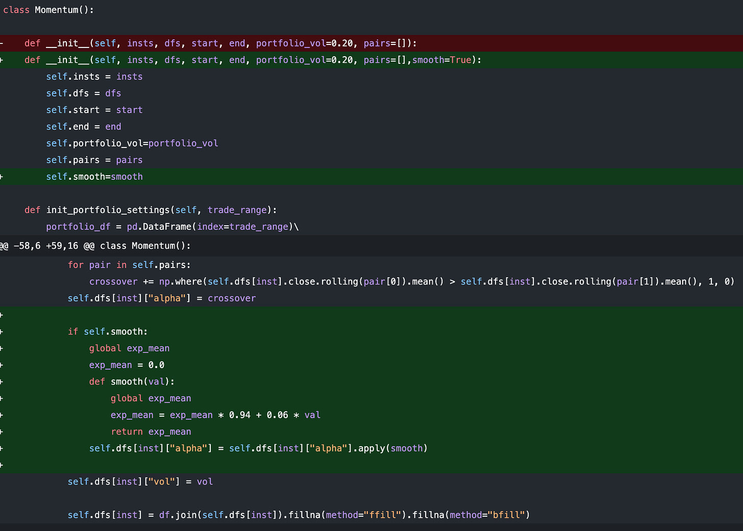
On the topic of costs…continuous signals are desirable. Instead of jumping in and out of large positions, continuity allows position to be scaled in and out of in a more balanced manner. The things we talked about help us precisely in this aspect. Another common technique is to smooth the forecast itself of the model under question. Perhaps not the most enlightening example, but on the trend following model:
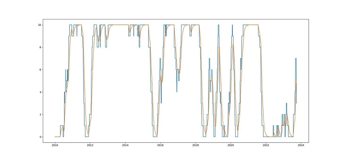
and the signals we get would look something like this, with the orange being the smoothed out version of the discrete blue signals.
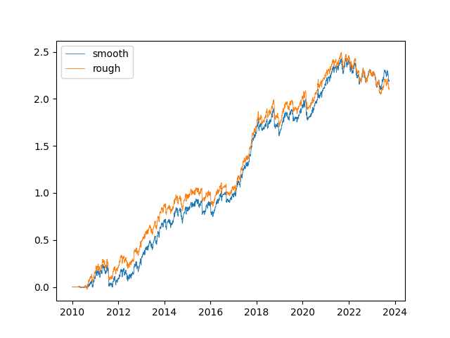
As I said, the signals here are highly correlated, so the trading performance pre-cost would not be particularly different:
but because of the curvature of the smoothed signals around some of the intermittent jumps in position sizing, there is good likelihood that the smoothed variant incur significantly less transaction costs, by which the difference might be noticeable.
We will leave the commentary here for now…again, do watch the QT101 lectures:
https://hangukquant.thinkific.com/courses/qt101-introductory-lectures-in-quantitative-trading
and there we will cover how we go from the code base attached to an alpha module that runs up to more than 100 times faster by being more CPU efficient.
See you in the next post. Code attachment (paid):


