In the last post:
we did a line-by-line walkthrough of the alpha simulator, using a uniform random variable to represent the signal generating component of the alpha backtest. We also raised a few questions:
How can we manage the varying levels of risk profiles of different stocks in our asset universe at a snapshot in time?
How can we manage the time varying levels of risk profiles of the entire portfolio across time?
How can we express a more nuanced view of the market? If we don’t have a continuous model, how can we still do this?
In this post, we will extend the alpha code implemented in the previous lecture to trade on a simple moving average crossover trend following strategy. We will then use this rule instance to address the first two questions. The changes to the code will be very minimal, so once you understand our last post - everything here follows. As before, the code is downloadable at the end of the post for paid readers.
Since there are minimal changes to the code, we will highlight the changes we need to make.
First, we create a trend.py file, and copy and paste the entire alpha.py code into it. Then in the main.py file, the following changes are made:
We then go back to the trend.py file and change the class name from Alpha to Momentum (which I am now realising is a misnomer). The rule we want to implement is a simple moving average crossover between the 10-day and 50-day pair. If the mean of the last 10 day closing prices are greater than the mean of the 50 day closing prices, we want to be long, otherwise we want to be flat. This is said to be a long-biased directional trend following rule. The intuition is that assets that are doing well now should do well in the future, but we don’t want to be short, since equities are in general, positive return bearing assets.
We make an aside here - as is, there is no way to distinguish between how `trendy’ our asset prices are at this point, since the rule is an indicator function. The crossover rule is a simple yes-no question represented by a single bit of information. To encode this rule, we will add just two lines to the compute_meta_information function in class Momentum:
Recall that in the previous post, we used a signal from a random number generator - here we let the alpha signals take the 1 and 0 values from our crossover.
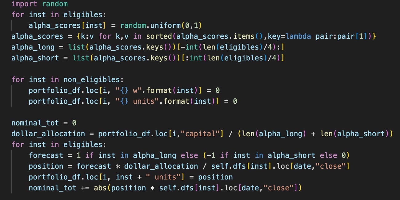
The natural question that arises is how we may translate these binary values into position sizing for our portfolio allocation. Since we are indifferent to the magnitude of trend but only to the presence of one (based on our 1-bit signal), all else equal, our approach is simple: allocate even amount of capital to all opened positions. Changing from the previous code block with random signals, our code now changes as follows:
We should be able to run the simulation now;
If you run the code - you will realise that the leverage is fixed to 1 (or 0 if no assets are trending):
Let us bring up the first question we want to answer:
How can we manage the varying levels of risk profiles of different stocks in our asset universe at a snapshot in time?
Now suppose you are at casino and there is a game where you believe you have an edge. In both games, you believe the outcome is an unbiased coin flip. In Game A, you get 12 bucks when you win and pay 10 when you lose. Here, your EV is +1. In Game B, you get 7 bucks when you win and pay 5 when you lose. Your EV is also +1. The game is no-limit, and you get to borrow at zero cost. Should you be indifferent to playing either game?
The answer is no, since the EV only captures the central tendency of your expected returns. The other artefacts of return distribution matters. Now in Game B, if you take twice as large bets as you otherwise would, then the W/L goes from (+7/-5) to (+14/-10). You are risking 10 bucks to make 14, as opposed the 12 bucks in Game A. This is because Game A’s natural stakes have 11 bucks standard deviation, and Game B’s natural stakes have 6 bucks standard deviation.
The standard deviation scales proportionate to leverage, so your EV compensation in Game A needs to scale for the player to be indifferent to playing either game.
What we are in fact looking for is a measure of risk-adjusted returns. We want to exactly quantify the statistic representing indifference between choices in terms of the outcomes in this play-game. To do that, we present a new Game \bar{A}, which has natural stakes (+14/-10). Then clearly betting twice in Game B is same as betting once in Game \bar{A}. Let’s create two candidates for risk-adjusted returns, namely the EV divided by variance and standard deviation. Make some computations:
It turns out that the indifference quantity is represented by the expected value divided by the standard deviation of the outcomes. This shall therefore determine the size of our bets, in the trend strategy. We don’t have an exact quantification on the EV, or even an approximation of it, but it does not matter to the relative sizing since our signal is uniformly one or zero.
Let’s try to implement that now…first, we assume we have some target volatility, then we will compute the volatility for each instrument using a thirty day window of standard deviations. Since we are taking positions with volatility as the denominator, in order to prevent positions from blowing up as it approaches zero, we will set a volatility floor at 0.005.
Now, we can use the volatility to size positions. We make the following changes:
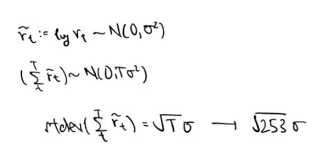
The volatility target passed in at 0.20 was annualised. The vol target variable is the volatility in daily terms presented in dollar units. To see this, consider a log return graph with the later half erased out.
The further out in time we traverse the graph for approximating the cumulated returns, the wider our estimation bands have to be in order for us to be reasonably confident. This is because the returns have random variance which accumulate. Assuming the returns are independently sampled, there are 253 trading days in a year, so to convert between daily and yearly variance/standard deviation requires some simple mathematics:
So instead of specifying our budget in terms of the portfolio capital, we are going to be specifying our budget in dollar volatility terms. The vol target variable is our volatility budget today in dollar terms. The forecast is scaled by the total number of forecasting chips bet, scaled to < 1 (assuming at least two assets are traded), then multiplying this by the vol target variable gives us the volatility budget scaled to a particular position. Now, we can simply divide this by the volatility budget consumption of a single contract to arrive at the position sizing.
Okay we can then run this:
and you might think…why did we perform worse (in terms of the terminal capital) after our risk management? Well, first, that is the wrong question to ask - risk management is not about maximising terminal wealth - that is under the purview of portfolio optimization. Secondly, that would be akin to arguing that Game A is better than Game B - it is not an apples to apples comparison, since our leverage is no longer fixed to one:
So we just answered the first question…what about the second?
How can we manage the time varying levels of risk profiles of the entire portfolio across time?
To answer this question, we can adopt the same principle. First, let us have a more nuanced discussion - although leverage, the degree of nominal exposure relative to capital, can be considered as a measure of risk, leverage inadequately measures the risk profiles of varying strategies. For instance, a fully invested portfolio in a basket of stocks is not the same risky as a full investment in a single stock, which is also not the same risky as a fully invested long-short market neutral portfolio.
Standard deviation, while imperfect, helps to alleviate these issues a little. There are no doubt other measures, but standard deviation is simple, easy to compute and easy to understand.
Now we know how much we want to bet on a relative scale, but we do not know how much we want to bet on an absolute scale. This is answered by the question we are now facing. Since we have already determined the measure of risk as standard deviation, we have two sub-questions: how much risk do we want, and how do we achieve that level of risk?
The first question is abit of a tricky one: the answer is that it depends. Some considerations are the investor mandate, risk preference, financial status, utility curve and skill, as well as the considerations presented mathematically in relation to the practical constraints outlined. Since the question is philosophical, we will not address most of it…and that of which is answered by mathematics are outlined in some of our previous posts:
So we are going to work with the assumption that we know beforehand the amount of risk we are willing to consume, which we argued is the standard deviation of returns, or equivalently, volatility. In this case, we assume that we want to consume 20% of annualised target volatility.
We can simply do this by keeping track of how much we are betting, the volatility realised from the betting that we have been doing, and then scaling our betting sizes going forward based on the target volatility in relation to the achieved volatility.
Adding these few lines to compute annualised vol for the current strategy:
we get » 0.1444560166092462 «
So we are undershooting the level of desired risk. To make the necessary sizing adjustments, we make the changes as follows in the Momentum class:
We make a function call to get_strat_scaler here:
We keep track of the realised volatility of portfolio returns using an exponentially weighted moving average, as well as the scalars used to achieve said return volatility. The get_strat_scaler function accordingly adjusts relative to target, and positions are scaled laterally by this scalar.
This is the achieved volatility and simulation results:
That is it! In the next post, we answer the third and final question that allows us to express our ideas of relative EV:
How can we express a more nuanced view of the market? If we don’t have a continuous model, how can we still do this?
Code zip (change .cbz extension to .zip and unzip): (paid readers)


