quantpylib.hft trade imbalance demo
After showcasing the hft backtesting lib, we used the modeller class to show effects of VAMP, one of the fair price estimators using order book features in short term price prediction:
Here we want to showcase another use of the same modeller class, this time modelling non-orderbook dynamics. In particular, we will demonstrate a trade imbalance study using quantpylib.
Trade imbalance is a simple idea - alot of buying in recent times imply excess demand and likely, future price upticks. It can be a feature in fair price estimation, but a mathematical model needs to be proposed to make fair price estimates from a TI estimate. The idea is simple; short term lop-sided trading on the bid or ask side are likely to lead to further price moves in the same direction. Here is the definition from the VAMP paper:
A positive correlation is assumed between the trade imbalance and mid price changes, to reflect demand for the asset when there is trend of market bids. The gamma weight decay gives more weightage to recent trades.
However, this formula is unsatisfactory for a number of general purposes. First, if there is consensus that information decay exists; then there serves no specific reason as to why such decay should not be applied to higher resolutions within each aggregated interval.
This may be a trivial concern for second intervals. A bigger issue is that the trade imbalance would be jumpy, or inestimable in the case of illiquid markets where trades occur at infrequent intervals - this is a given in many crypto pairs. For example, one buy two minutes ago, and then one sell a minute later would give trade imbalance figures: -1,1 respectively. One may attend to this by widening the interval at which trades are aggregated - for which then the issue waved trivial earlier is no longer so. Imagine an aggregation interval of five minutes: a buy and sell order in the most recent interval 4.59m ago and another 0.01m ago contain significantly different amount of priced-in 'information' to market participants.
That there should be a decay is almost undisputed in finance. Nature of decay, and whether the decay should be w.r.t to trade arrivals in numbers, time distance or some other axis is philosophical. We propose a generalized estimator:
The aformentioned TI formula would be a specific instance of this generalization, where n = number of trades within x seconds, and omega is a piecewise constant decay function.
Again, let's load the same dataset:
from quantpylib.utilities.general import load_pickle

(
    ob_timestamps,
    bids,
    asks,
    mids,
    trades
) = load_pickle("hft_data")

import numpy as np
import matplotlib.pyplot as plt
from pprint import pprint
from quantpylib.hft.alpha import EVENT_CLOCK, EVENT_LOB, EVENT_TRADE
from quantpylib.hft.alpha import Model
from quantpylib.hft.utils import rolling_apply
from quantpylib.hft.features import trade_imbalance

class TI(Model):

    def compute_trade_features(self,trade_buffer):
        pass

    def event_estimator(
        self,ts,event_type,event_id,type_id,
        trade_buffer,ob_timestamps,ob_bids,ob_asks,ob_mids,features,
        running_event_ids,running_type_ids,**kwargs
    ):
        pass
This time, the feature is trade-related. So we will pre-process the TI estimates and then make estimates on each EVENT_TRADE. We can do this using the quantpylib.hft.utils's rolling_apply function that does what the name-suggests, on rolling numpy array samples:
    def compute_trade_features(self,trade_buffer):
        tis = rolling_apply(a=trade_buffer,window=20,func=trade_imbalance)
        return {
            "TI":tis
        }
The trade-imbalance from quantpylib.hft.features has implementation like this:
def trade_imbalance(
    trades,
    decay_function=lambda sample: exponential_weights(arr=sample,unique_values=True,normalize=True),
    window_n=None, window_s=None, T=None
):
    if T is not None: trades = trades[trades[:,0] <= T]
    if sum(1 for param in [window_n,window_s] if param is not None) > 1:
        raise ValueError("sample window can only be defined by one of window_n, window_s")
    if window_n is not None :  trades = trades[-window_n:]
    if T is None: T = trades[-1,0]
    if window_s is not None: trades = trades = trades[trades[:, 0] >= (T - window_s*1000)]

    #trade = ts, price, size, dir
    if len(trades) == 0: return 0
    weights = decay_function(T - trades[:, 0])
    signed_volume = trades[:, 2] * trades[:, 3]
    return np.sum(weights * signed_volume) / np.sum(weights * trades[:, 2])
refer to implementation of exponential_weights in the repository code; or use your imagination. We just used the last twenty trade events, but of course this is up to you. Making estimates are simple, we just echo this at the correct event:
    def event_estimator(
        self,ts,event_type,event_id,type_id,
        trade_buffer,ob_timestamps,ob_bids,ob_asks,ob_mids,features,
        running_event_ids,running_type_ids,**kwargs
    ):
        estimates = {}
        if event_type == EVENT_TRADE:
            estimates['TI'] = features[EVENT_TRADE]["TI"][type_id]
        return estimates
Running it is even simpler:
alpha = TI(
    ob_timestamps=ob_timestamps,
    ob_bids=bids,
    ob_asks=asks,
    ob_mids=mids,
    trade_buffer=trades,
)
alpha.run_estimator()
In this case TI just ranges from -1 to 1 - it is not yet a fair price estimator. But we can ask for useful dataframes:
variable_df = alpha.df_estimators(include_forwards=True)which looks like this:
                     TI        t0        t1        t5       t15       t30       t60
1722092423332 -1.000000  0.202500  0.202340  0.202275  0.202275  0.202205  0.202255
1722092423534 -0.951384  0.202500  0.202345  0.202275  0.202275  0.202205  0.202255
1722092424342 -0.903858  0.202340  0.202305  0.202275  0.202275  0.202205  0.202255
1722092428167 -0.869708  0.202275  0.202275  0.202275  0.202275  0.202205  0.202250
1722092447111 -0.730021  0.202335  0.202305  0.202205  0.202245  0.202265  0.202315
...                 ...       ...       ...       ...       ...       ...       ...
1722095930541  0.784021  0.200680  0.200705  0.200740  0.200655  0.200775  0.200730
1722095933658  0.847519  0.200705  0.200685  0.200735  0.200635  0.200830  0.200710
1722095934190  0.805306  0.200755  0.200740  0.200730  0.200635  0.200830  0.200690
1722095938015  0.821895  0.200735  0.200730  0.200715  0.200470  0.200865  0.200730
1722095939023  0.696006  0.200730  0.200730  0.200675  0.200465  0.200900  0.200730
for each TI estimate at each trade event, we have preloaded a dataframe with the instantaneous mid price, and mid prices up to sixty seconds out.
Let's propose a fair price model using this TI figures. The model we choose should be determined by the average holding period - obviously if we are buying and selling out the position within one-second, the price in sixty seconds is less relevant.
We shall try a least-squares, zero-intercept simple regression model, with the help of our regression library quantpylib.simulator.models.GeneticRegression. This allows us to do things like
from quantpylib.simulator.models import GeneticRegression
regmodel = GeneticRegression(
    formula="div(minus(t1,t0),t0) ~ TI",
    df=variable_df,
    intercept=False
)
res = regmodel.ols()
regmodel.plot()
print(res.summary())
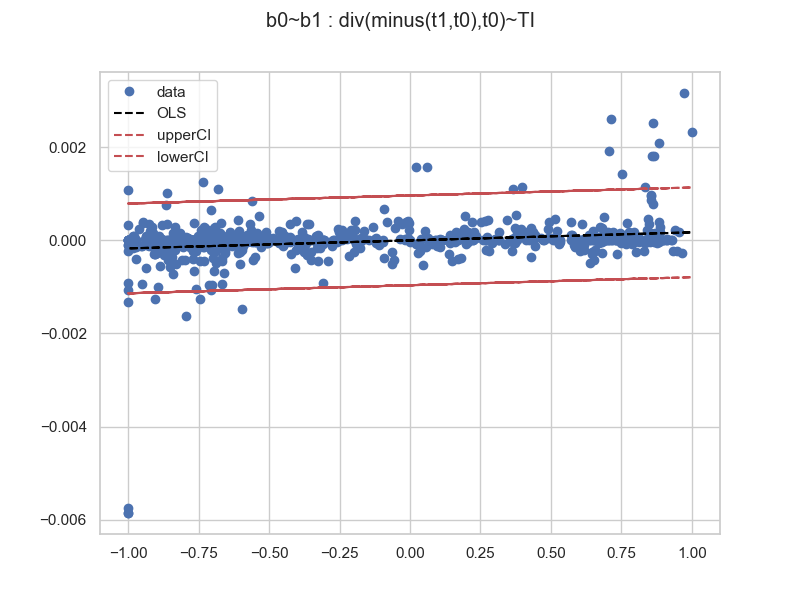
We get a bunch of useful plots - here is one:
with summary
                                 OLS Regression Results
=======================================================================================
Dep. Variable:                     b0   R-squared (uncentered):                   0.051
Model:                            OLS   Adj. R-squared (uncentered):              0.050
Method:                 Least Squares   F-statistic:                              44.43
Date:                Sat, 03 Aug 2024   Prob (F-statistic):                    4.81e-11
Time:                        18:56:51   Log-Likelihood:                          5116.2
No. Observations:                 825   AIC:                                 -1.023e+04
Df Residuals:                     824   BIC:                                 -1.023e+04
Df Model:                           1
Covariance Type:            nonrobust
==============================================================================
                 coef    std err          t      P>|t|      [0.025      0.975]
------------------------------------------------------------------------------
b1             0.0002   2.59e-05      6.666      0.000       0.000       0.000
==============================================================================
Omnibus:                      898.172   Durbin-Watson:                   0.984
Prob(Omnibus):                  0.000   Jarque-Bera (JB):           163861.949
Skew:                          -4.759   Prob(JB):                         0.00
Kurtosis:                      71.383   Cond. No.                         1.00
==============================================================================
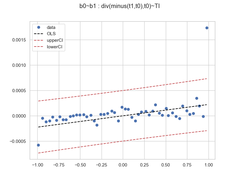
Statistically significant it says. Perhaps we would like to zoom out more and see some aggregated features. The GeneticRegression.ols allows us to bin data into blocks, and then aggregate the axis values. We will take defaults:
from quantpylib.simulator.models import Bin
regmodel.ols(bins=50,bin_block="b1",binned_by=Bin.WIDTH)
regmodel.plot()
and we see:
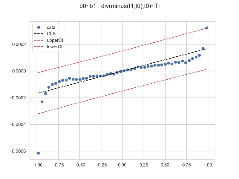
Here the sample size is 825. Let's do the regression on some 448228 trade data samples (collect your own data boys and girls), and then binned, regressed and plotted:
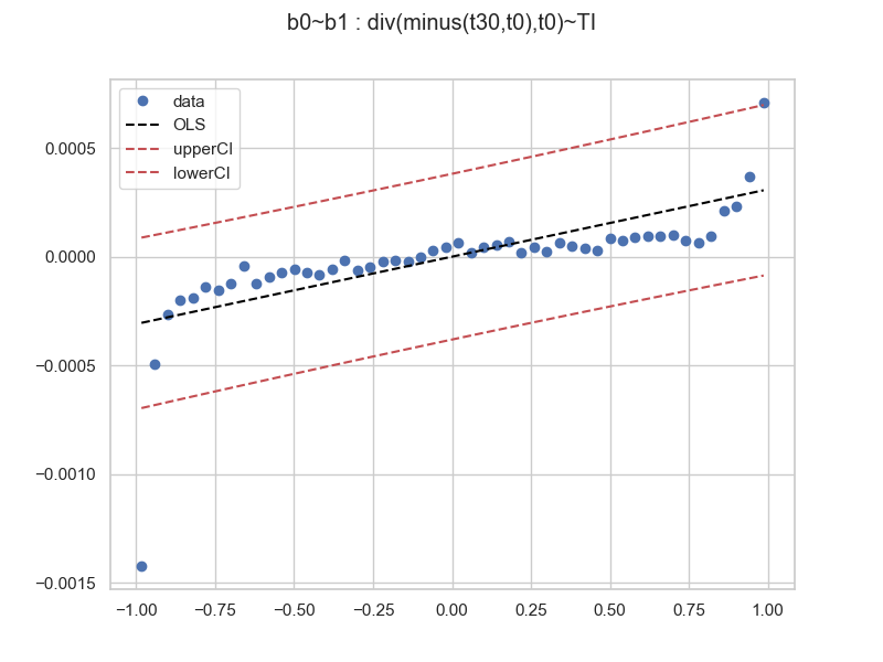
When more data samples are collected, here the trend is obvious. However, we can see that the residuals are non-random. The suggested relationships appears to be curvilinear. Perhaps a higher order polynomial (cubic?). We stop here, fit your own data! The tools have been provided. On the same 448228 size dataset, we try a longer prediction div(minus(t30,t0),t0) ~ TI and get
the result is similar.
Cheers. Quantpylib is meant for annual readers of HangukQuant:


