


dummy stoikov

Here, we give low resolution walk through of inventory handling in the market-making framework of Avellaneda & Stoikov (AnS). The paper is here:
https://people.orie.cornell.edu/sfs33/LimitOrderBook.pdf
Hummingbot has a blog post here:
https://hummingbot.org/academy-content/guide-to-the-avellaneda--stoikov-strategy/
and they have an implementation here.
We will assume the role of a dummy (actually, no assumption required on my end). Interestingly, the AnS implementation in the repo deviates from their blog post. We will cover some of these concerns, and then just reformulate the whole thing.
The AnS framework is useful in that it allows skewing of bid-ask quotes relative to held inventory, which decreases equity variance; a reasonable measure of risk. However, one should note that this is hardly `alpha` - narrowing the spread of a return distribution without changing the mean does little to help in pushing towards a profitable enterprise;
the going concern of managing inventory is secondary relative to the primary concerns of knowing how wide and when to skew, short-term fair price predictions and avoiding adverse fills.
Let’s begin. The AnS begins by determining some fair price s - here we can assume that the mid price is fair:
here the r is given terminology `reservation price`, and is an adjustment to the mid (fair) price by a additive factor scaled by inventory q. In the paper q is said to be number of stocks held. T is some terminal quoting time (say exchange close), t is current time. Gamma is some risk aversion parameter, that determines how aggressive we want to go towards zero inventory. It is really quite simple, if q > 0, then r is lower than fair price, so we shift our quotes parallel downwards so that the limit ask price is closer to top of book.
So quotes are placed around the reservation price. How-wide is determined by
Here the deltas are just (quote - r) distances, and we can assume symmetrical. So the distance between ask limit price and bid limit price is just given by the RHS. The risk-aversion parameter shows up, and the kappa value is a measure of orderbook liquidity. I wrote about that here:

where I also mentioned I am highly suspect of Hummingbot’s computation, particularly in that it is not normalized. This probably leads to the gamma problem later…as I will highlight
Here is a quote:
In practice I would not bother fitting the kappa estimator (at least not live anyway, I might fit it on historical data to get a feel for the base spread) due to the sample size required to get a non-noisy estimate, which would be too slow for updating my quotes.
Ok now I am going to talk about what Hummingbot changed.
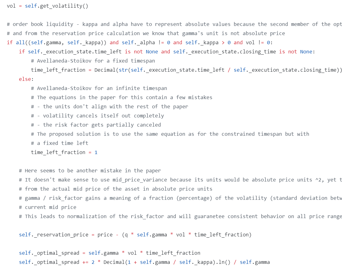
First, they argue that it does not make sense that the reservation price formula has a subtraction term that is in units of price^2. I don’t know, I haven’t done the math, but I have to say it does seem fishy. The first term is clearly in units of the stock price, and the subtraction is price^2. Kinda funky, and this has much better interpretations:
and then their adjustment to all-round quoting for crypto exchanges is to set (T-t) = 1, so instead we arrive
Okay, this I can understand. It tells me to adjust the fair/mid price by a factor of the price volatility, depending on risk-aversion and inventory levels.
The second equation tells us that how wide we quote is a function of volatility and order book liquidity. The liquidity is measured by fitting an exponential decay model to hit rate of limit orders placed at variable distances to mid - the more illiquid the book, the greater probability of getting hit or lifted wider - we also place our quotes wider.
At this point, the model is simple and intuitive enough that if we are able to calibrate these parameters accurately, we have a working framework about which we can manage portfolio inventory through risk level gamma.
Here are my objections.
I have tried to fit kappa and it is ridiculously noisy. Often this second term dominates how wide I quote, and is mostly noise. So, let’s just zoom out and look at what the terms are: very simple actually - just one term that says quote based on volatility, and another that says quote based on underlying liquidity of the order book. I am just going to go ahead and say that the second term can be eye-balled somewhat easily by just…looking at the damn order book spread. Obviously, illiquid tickers have larger base spreads to compensate market makers taking inventory risk. If we are going to manually decide on the liquidity parameter, AND the risk-aversion constant - the whole thing is just a scalar value.
where B is some base spread. Now, since you are going to decide this constant anyway, meaning you decide the scale - let’s just take out the superscripts:
Okay, this - even my monkey brain - can understand. Let’s make it even simpler, shall we. It would be nice if the remaining terms were easy to compute, but even here I can’t seem to find a consensus. For example, what is q? I have seen multiple interpretations - some say number of stocks held, others say dollar inventory relative to target inventory over max inventory, so on and so forth.
Let’s say we take q = (actual - target) / max. This means q is strictly < 1 ? Kind of seems weird. Number of stock also hardly seems to make sense. To make matters worse, let us take a look at what Hummingbot writes here:
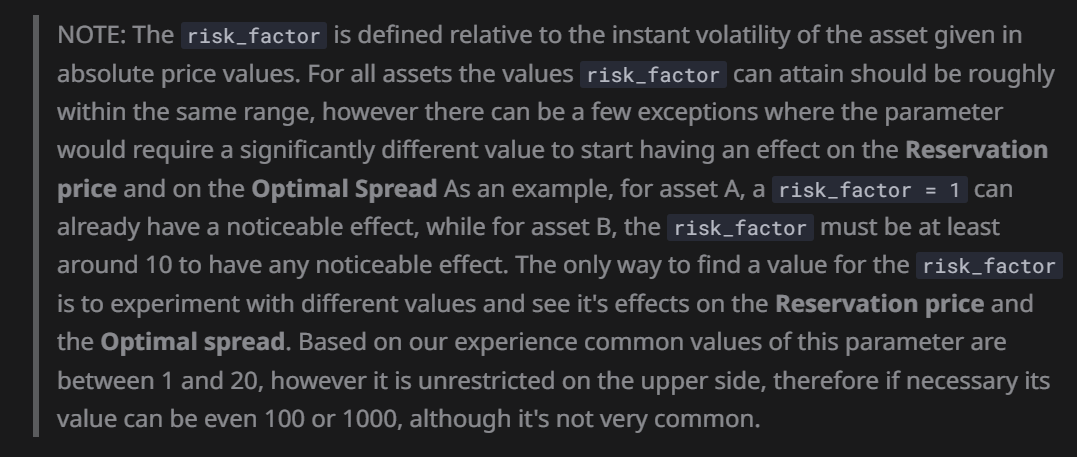
Huh? So gamma is now just supposed to be some value from 0 to 1000, and then I have to go figure this out myself? I don’t know, I am not smart enough to pick a right value from that range. I am going for intuition.
Now, the AnS model does not specify our order size either. Now imagine q was number of stocks: and our order size is 100. Now, our q goes like 100, 0, -100, -200, -100…hardly seems sensible either.
Let’s try to come up with a sensible function q. Maybe something like:
where order size value
Here, actual is the current dollar value of position held. target is the target dollar value to hold, and block is the user-determined value of a block of inventory. The block value is decided based on how aggressively we want to skew our quotes towards target inventory. For example, suppose we have actual = 100, target = 50, a block size of 50 would be q = 1, and a block size of 10 would be q = 5. The volatility of inventory level q is determined as a function of block size and zeta- here we have kept it general to some parameter zeta, but it may be something as simple as block/10 or something like that. It simply determines the fraction of block units each filled order should take us towards/away from current portfolio state. For instance, suppose again (100 - 50) / 50 = 1. If n = block, then one sell order immediately gets us to actual = target.
So the aggressiveness is now determined no longer by an obscure value, but by two variables - one that determines block distance, and the order size function that determines volatility about inventory q w.r.t. filled orders.
We don’t need gamma anymore:
and we replace gamma in the wide-ness equation with some tightness factor lambda:
so that large values of lambda correspond to a stink bid/ask and smaller values are tight quotes. We are now down to the essentials of the framework that allows us to manage inventory. We have to decide on a few inputs:
block, order size » determines aggressiveness and volatility of inventory q
sigma, calibrated from market
B, the base, minimal spread absent price volatility
lambda, how tight we quote on estimate volatility
We butchered the entire econophysics theory, but at least it works. Almost as importantly, we understand it.
No geniuses were harmed in the writing of this post.
*not use
finally, this paper does use the “reservation price” model but just give the optimal spread on the bid and in the ask, but you can compute a reservation price with a bit of maths and both approaches are exactly the same at the end.