quantpylib.hft.trades/features/stats

Few days (well, yesterday) ago, our documentation on the limit-order-book was live:

quantpylib.hft.lob documentation live; and more

Now the internal trade buffer and statistics library is up. We will definitely add more functionalities to this in the weeks to come. We have a nice example, and we will demonstrate how the different components work in this post, through the example of measuring order book liquidity; a similar example is implemented in the Hummingbot trading intensity estimator, but our code uses slightly different logic.

To compute orderbook liquidity - we fit an exponential decay model for the hit and -lifted amounts against the distance to mid price. This figure is directly related to the Poisson intensity that is often taken as a model for trade arrivals.

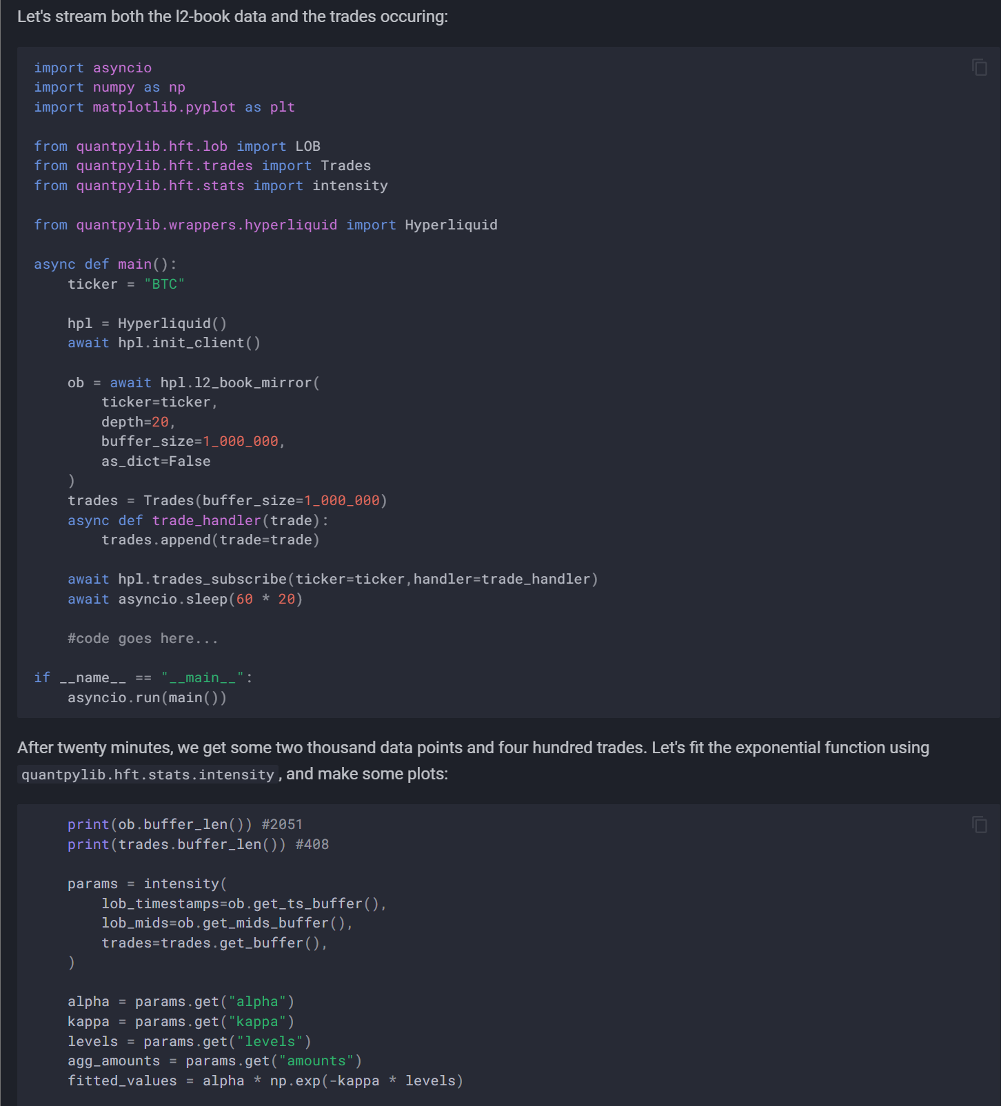
Let's stream both the l2-book data and the trades occuring:

import asyncio
import numpy as np
import matplotlib.pyplot as plt

from quantpylib.hft.lob import LOB
from quantpylib.hft.trades import Trades
from quantpylib.hft.stats import intensity

from quantpylib.wrappers.hyperliquid import Hyperliquid

async def main():
    ticker = "BTC"

    hpl = Hyperliquid()
    await hpl.init_client()

    ob = await hpl.l2_book_mirror(
        ticker=ticker,
        depth=20,
        buffer_size=1_000_000,
        as_dict=False
    )
    trades = Trades(buffer_size=1_000_000)
    async def trade_handler(trade):
        trades.append(trade=trade)

    await hpl.trades_subscribe(ticker=ticker,handler=trade_handler)
    await asyncio.sleep(60 * 20)

    #code goes here...

if __name__ == "__main__":
    asyncio.run(main())

After twenty minutes, we get some two thousand data points and four hundred trades. Let's fit the exponential function using quantpylib.hft.stats.intensity, and make some plots:

    print(ob.buffer_len()) #2051
    print(trades.buffer_len()) #408

    params = intensity(
        lob_timestamps=ob.get_ts_buffer(),
        lob_mids=ob.get_mids_buffer(),
        trades=trades.get_buffer(),
    )   

    alpha = params.get("alpha")
    kappa = params.get("kappa")
    levels = params.get("levels")
    agg_amounts = params.get("amounts")
    fitted_values = alpha * np.exp(-kappa * levels)

    # Plot the actual and fitted
    plt.figure(figsize=(10, 6))
    plt.plot(levels, agg_amounts, 'o', label='Aggregated Amounts', color='red')
    plt.plot(levels, fitted_values, '-', label=f'Fitted Model: $A(d) = {alpha:.2f} e^{{-{kappa:.2f} d}}$', color='blue')
    plt.xlabel('Distance from Mid-Price (d)')
    plt.ylabel('Aggregated Trade Amount (A(d))')
    plt.title('Exponential Decay Model Fit to Aggregated Trade Amounts')
    plt.legend()
    plt.grid(True)
    plt.show()

Obviously, the sample size is rather small, but we will carry on for the sake of demonstration. Here is the decay function:

Values such as kappa are often used as measures of orderbook liquidity. Higher values of kappa indicate strong decay, hence greater trading near the mid-price. Lower values indicate weak decay - market order sizes often wipe out a few levels in the orderbook and have strong price impact. See Hummingbot implementation of computing trade intensity. In stoikov-avellaneda market making formula, kappa appears as term in optimal spread; see Hummingbot avellaneda_market_making.pyx:

self._optimal_spread = self.gamma * vol * time_left_fraction
self._optimal_spread += 2 * Decimal(1 + self.gamma / self._kappa).ln() / self.gamma

Optimal spread has an additive factor of log(1 + c/kappa), where smaller values of kappa encourages wider maker orders (although I am pretty sure this should be dollar-normalized first).

Anyhow, this shows how the trades, lob and statistics module in the quantpylib.hft can be used together. In practice I would not bother fitting the kappa estimator (at least not live anyway, I might fit it on historical data to get a feel for the base spread) due to the sample size required to get a non-noisy estimate, which would be too slow for updating my quotes.

Cheers~