Sketching the Option Backtester (with Code downloadable for ALL readers)

..preview..

A few days ago…we did our market notes:

Rounding up Convex Opt (Market Notes, 891 pages)

Time for some programming. We begin off with writing simple code for option/volatility trading, and to test our ideas. We want to follow the same structure as the Russian Doll, which allows for hyper-efficient (in a Pythonic way) testing of quantitative strategies. But since we are trading derivative contracts, each underlying with an option chain - this presents massive challenges.

For those who want to see the tester on linear, continuous contracts, our free and introductory quant course covers the basics of the Russian Doll:

https://hangukquant.thinkific.com/courses/qt101-introductory-lectures-in-quantitative-trading

The majority of the challenges are with reference to the added dimensionality of the data - before this, we had time and asset considerations. With the option chain, there are minimally two additional dimensions (the term structure and the strike) we have to consider; where in the volatility surface do we want to pick our contracts?

With minimally FOUR dimensions, the vectorisation approach is quite impossible, in both logic design and efficiency. We will address this. Another is the data - in the testing for crypto/equity products, we could just preload 20years of data into RAM, mostly without worrying if the application will crash. It won’t work on option testing.

But as always, we begin with a simple model, and then we iterate to a better solution. Make it work…then can it be better?

Here, we will just make it work. Simple - one contract, simple rule, just compute the pnl of a short ATM straddle on 3x notional exposure moderately close to expiry. Enough talk…let’s get dirty.

Our option data reference for this post is https://historicaloptiondata.com/ ‘s L2 ALLSPX - we are unaffiliated with them. The data is not free. You can use your own datasets, and the code we design should not be specific to which dataset provider you use.

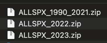
So I save them all in a folder, and the zipfiles look like this

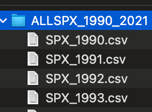
If I unzip they look like this:

but we will keep it zipped, and if you open the csv file in Excel, you get something like this:

Ok so now you know how the data is structured, let’s write the code. The code is downloadable at the end of the post for all readers, so we will just highlight comments. Once the volatility series is done, I will push the changes to the community Github, which paid readers have repo access. For those who want an in depth thought considerations and how I engineered the final engine, I will stream a quant lecture.

Starting with some imports

import os
import pytz
import zipfile
import pandas as pd 
import numpy as np

from datetime import datetime
from collections import defaultdict
from dateutil.relativedelta import relativedelta

we let the main engine run

async def main():
    tickers = ["SPX"]
    trade_start = datetime(2000,1,1,tzinfo=pytz.utc)
    trade_end = datetime(2023,6,1,tzinfo=pytz.utc)
    optstrat = OptAlpha(
        instruments=tickers,
        trade_range=(trade_start,trade_end),
        dfs={}
    )
    df = await optstrat.run_simulation()
    import matplotlib.pyplot as plt
    plt.plot(df.capital)
    plt.show()
    
if __name__ == "__main__":
    import asyncio 
    asyncio.run(main())

so…OptAlpha?

class OptAlpha():
    
    def __init__(self,trade_range,instruments=[],dfs={},portfolio_vol=0.20):
        self.trade_range = trade_range
        self.instruments = instruments 
        self.dfs = dfs 
        self.portfolio_vol = portfolio_vol  

so far so normal. Run simulation? We don’t even have data loaded yet, as you can see from our OptAlpha object initialisation. Because loading it would likely exceed RAM. So we will load it in the run simulator:

    async def run_simulation(self):
        self.instantiate_variables()
        trade_start = self.trade_range[0]
        trade_end = self.trade_range[1]
        trade_range = pd.date_range(
            start=datetime(trade_start.year, trade_start.month, trade_start.day), 
            end=datetime(trade_end.year, trade_end.month, trade_end.day),  
            freq="D",
            tz=pytz.utc
        )
        self.compute_metas(index=trade_range)
        
        portfolio_df = pd.DataFrame(
            index=trade_range
        ).reset_index().rename(columns={"index":"datetime"})
        portfolio_df.at[0,"capital"] = 100000.0
        last_positions = self._default_pos()
        positions = {}
        #to be continued


    def instantiate_variables(self):
        self.data_buffer=[]
        self.data_buffer_idx=[]
        self.unzipped,self.loaded=set(),set()

    
    def compute_metas(self,index):
        return 

these look familiar, if you have gone through the Russian Doll. What are the variables for the data buffer, data buffer index and so on? These are specific to how you want to load, from your own database - which you should define accordingly to your own data schema.

Our critical data structure is just going to be two lists. The first list contains elements which are all the option data relevant to a particular trading day, and the second list contains elements which is the date pointing to the corresponding dataframe in the former list.

The signal dictionary looks like this:

    def _default_pos(self):
        return defaultdict(lambda : {
            "S":0,"C":[],"P":[],"CU":[],"PU":[]
        })

for any option strategy, we will trade in the underlying, and arbitrary number of legs in calls and puts. The rest of the run simulator looks like this:

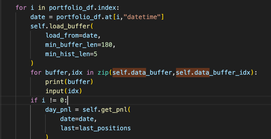
        for i in portfolio_df.index:
            date = portfolio_df.at[i,"datetime"]   
            self.load_buffer(
                load_from=date,
                min_buffer_len=180,
                min_hist_len=5
            )  
            if i != 0:
                day_pnl = self.get_pnl(
                    date=date,
                    last=last_positions
                )
                print("pnl",day_pnl)
                portfolio_df.at[i,"capital"] = portfolio_df.at[i-1,"capital"] + day_pnl
            
            signal_dict = self.compute_signals(date,portfolio_df.at[i,"capital"])
            signal_dict = signal_dict if signal_dict else last_positions

            positions[date] = signal_dict
            last_positions = signal_dict
            if i % 50 == 0: print(portfolio_df.at[i,"capital"])
        return portfolio_df

so we just have to figure out what goes in the load buffer, and what goes in the signal compute.

To demonstrate, I print the dataframes after the load_buffer

each element is just the dataframe I screened and the quote date. How you obtain this is completely dependent on where you store your data and the data structure of your data source, so it is not that important, and you may read the source code attached.

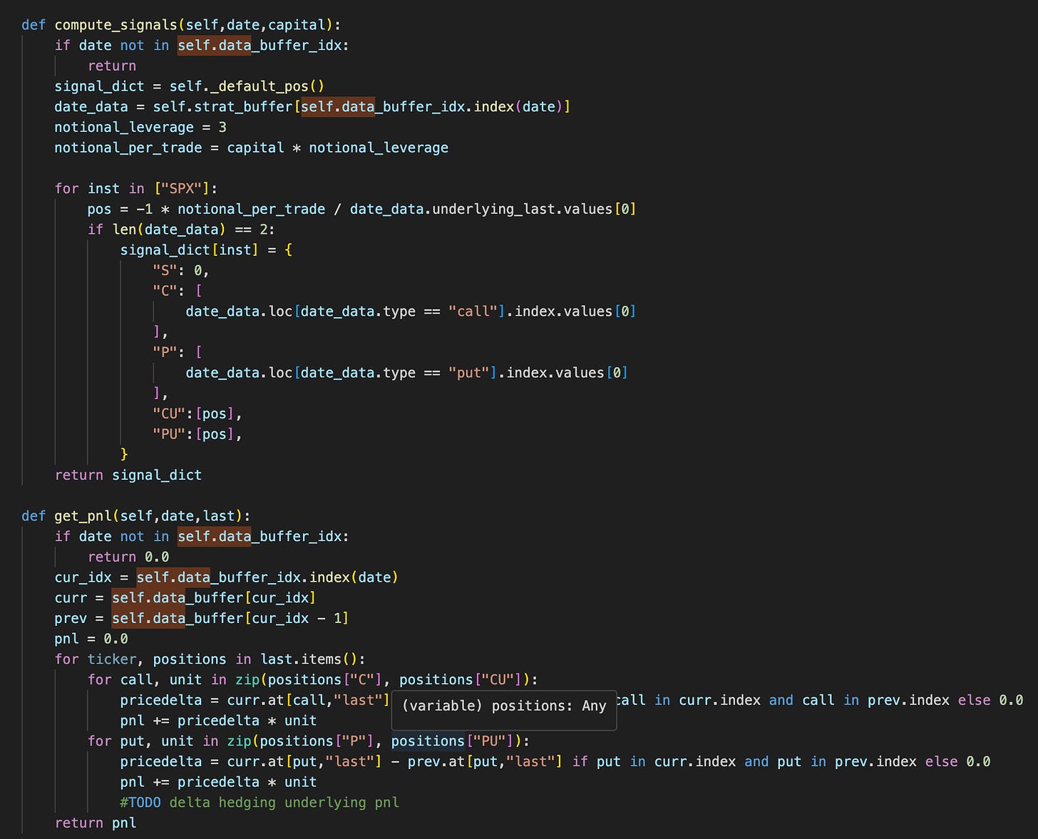
Just the pnl and signal computation is left:

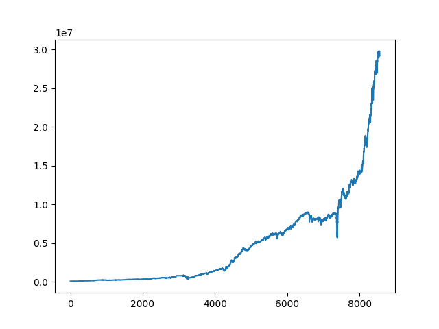
We run the code, and here is the pnl graph:

which is unsurprising, since we already know that index options are overpriced due to the variance premium.

But on a more important note, the code here is not particularly flexible, and is also highly efficient.

But we will stop here for now - in the next post, we will try selling straddles on single stock equities, to make it clear what would be the common code features when faced with different data structures and rules. We will explore the shortcomings, and this will help us identify the problem points to iterate towards a better quant volatility testing engine.

Code (download as usual, change cbz extension to zip):

Code

2.74KB ∙ CBZ file

Read now

Read now