Dual Momentum in Cryptocurrencies?

Over the last few weeks, we talked about funding arbitrage,

extended the quant library to incorporate crypto backtesting

and introduced new features for regression analysis:

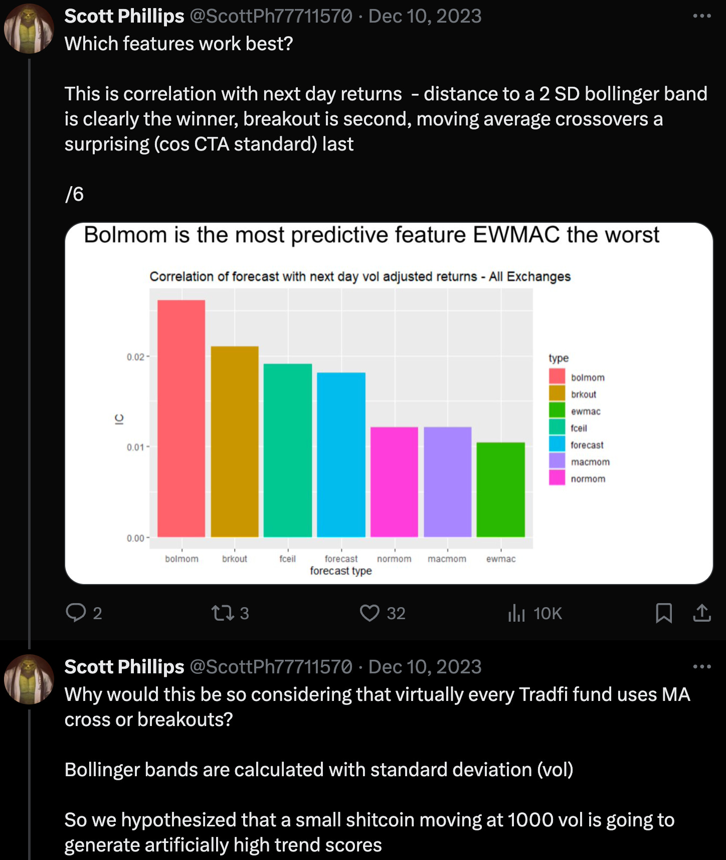
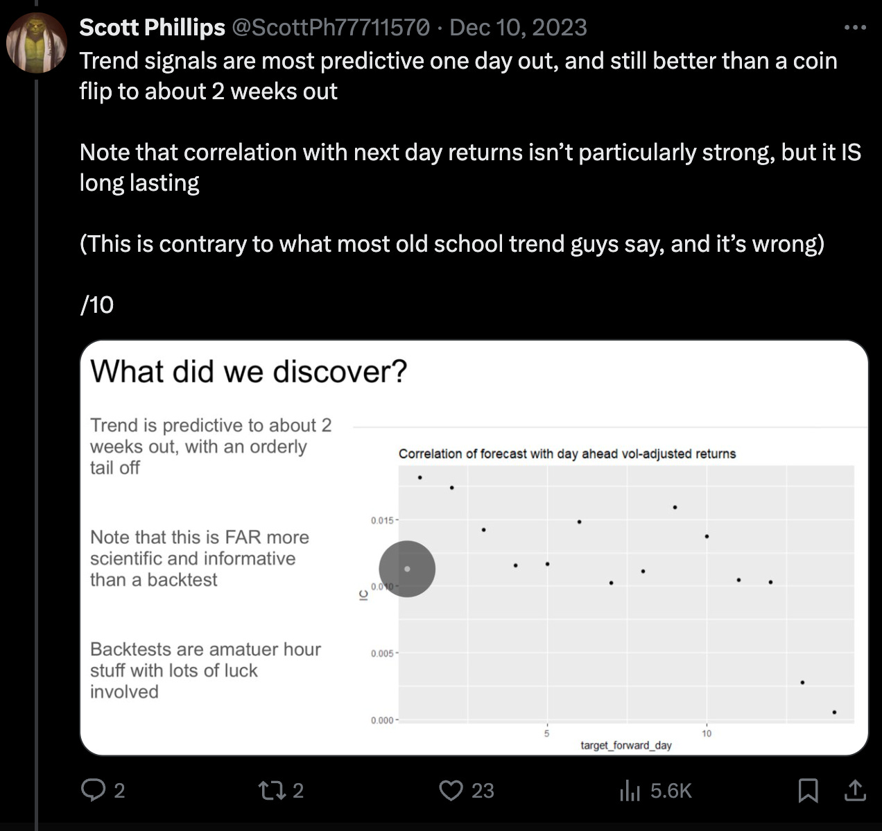
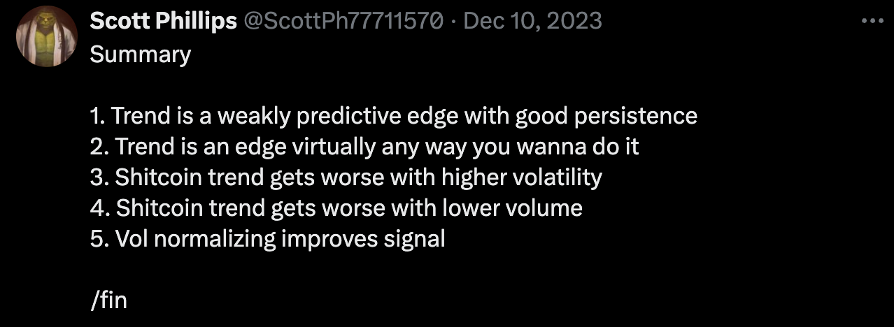
It only seems fitting we use some of these features to talk about strategies in the cryptocurrency market. Today, it will be trends, trends everywhere. We will be analysing stuff, verifying stuff and plotting stuff, with code. Here is an excellent thread on trends in coin markets:
https://twitter.com/ScottPh77711570/status/1733690323946414377
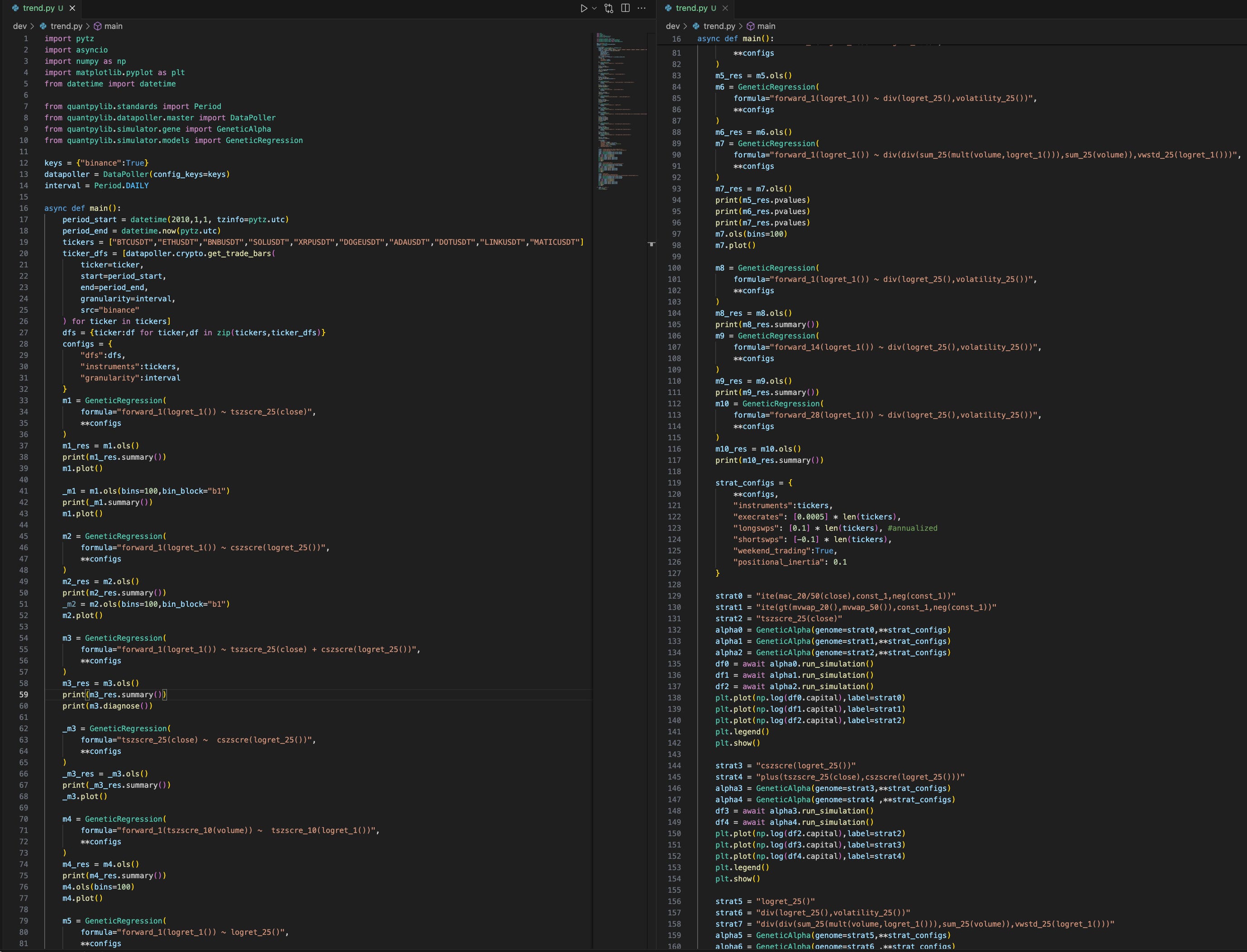
Let’s begin by obtaining some data, for 10 of some of the largest crypto coins:
import pytz
import asyncio
import numpy as np
import matplotlib.pyplot as plt
from datetime import datetime

from quantpylib.standards import Period
from quantpylib.datapoller.master import DataPoller
from quantpylib.simulator.gene import GeneticAlpha
from quantpylib.simulator.models import GeneticRegression

keys = {"binance":True}
datapoller = DataPoller(config_keys=keys)
interval = Period.DAILY

async def main():
    period_start = datetime(2010,1,1, tzinfo=pytz.utc)
    period_end = datetime.now(pytz.utc)
    tickers = ["BTCUSDT","ETHUSDT","BNBUSDT","SOLUSDT","XRPUSDT","DOGEUSDT","ADAUSDT","DOTUSDT","LINKUSDT","MATICUSDT"]
    ticker_dfs = [datapoller.crypto.get_trade_bars(
        ticker=ticker,
        start=period_start,
        end=period_end,
        granularity=interval,
        src="binance"
    ) for ticker in tickers]
    dfs = {ticker:df for ticker,df in zip(tickers,ticker_dfs)}
    configs = {
        "dfs":dfs,
        "instruments":tickers,
        "granularity":interval
    }
What model should we begin with?
Ok cool, so let’s regress forward returns against bollinger score (z-score of closing prices).
    m1 = GeneticRegression(
        formula="forward_1(logret_1()) ~ tszscre_25(close)",
        **configs
    )
    m1_res = m1.ols()
    print(m1_res.summary())
    m1.plot()
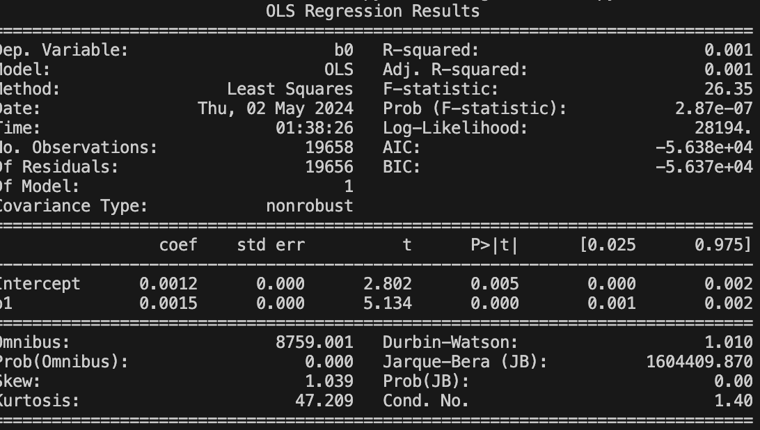
The bollinger-score is statistical significant, but the plots are abit murky to interpret, what with almost 20000 data points. Also it is financial data..of course there are going to be outliers:
Most market `effects` are slight edges - if they were too pronounced, they would cease to exist in the first place. Let’s mute out the noises by binning the bollinger-score axis into 100 intervals of equal number of observations, and then taking the winsorized mean (the default aggregator in ols).
_m1 = m1.ols(bins=100,bin_block="b1")
print(_m1.summary())
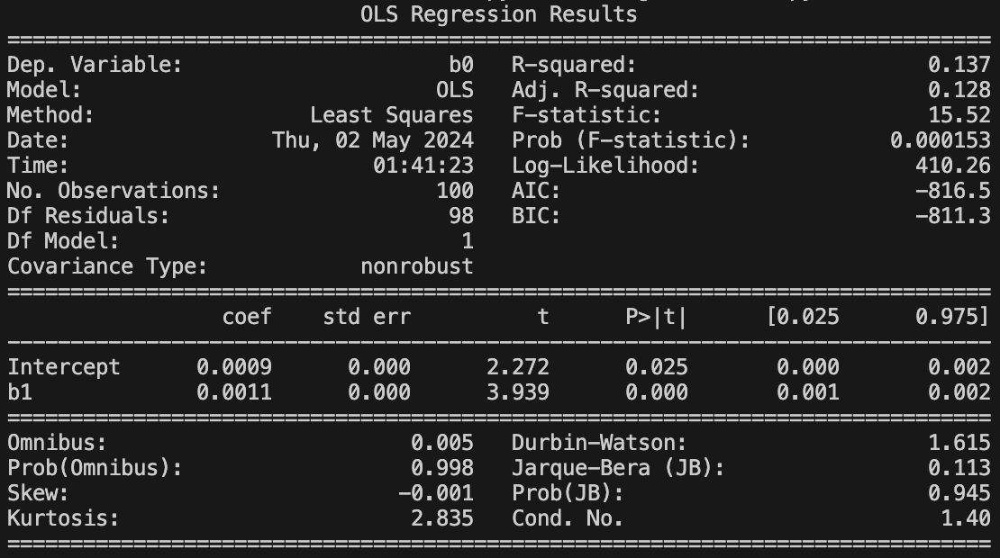
m1.plot()Our plots are much cleaner:

and the regression tests draw the same conclusion:
From now, we will present regression results in non-aggregated context and regression plots in the aggregated form, where the aggregation function follows winsorization of 0.05 quantiles at both ends.
Okay, so the data suggests trend following (time-stickiness of outperformance) exists in cryptocurrency data.
What about momentum (cross-sectional stickiness of outperformance)?
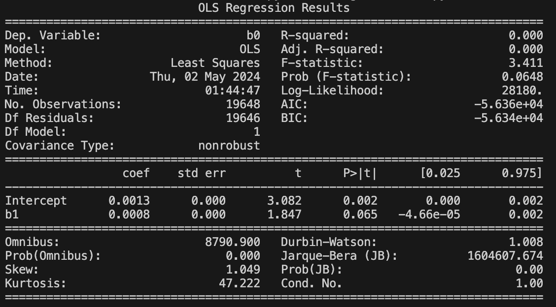
    m2 = GeneticRegression(
        formula="forward_1(logret_1()) ~ cszscre(logret_25())",
        **configs
    )
    m2_res = m2.ols()
    print(m2_res.summary())
    _m2 = m2.ols(bins=100,bin_block="b1")
    m2.plot()
Here is the regression result:
and diagnostic plot:
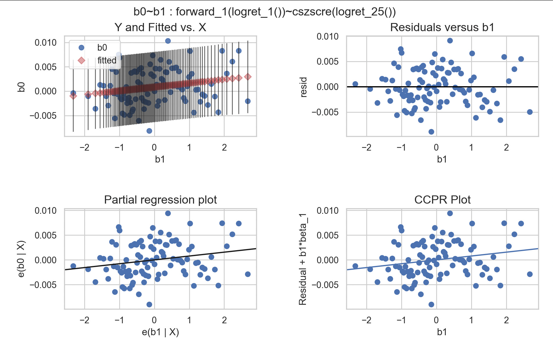
Momentum also, although of a less significant concern than trend-following, is somewhat statistically significant in predicting forward one-day returns.
Then, should a portfolio incorporate both (dual momentum)? We can apply multivariate regression:
    m3 = GeneticRegression(
        formula="forward_1(logret_1()) ~ tszscre_25(close) + cszscre(logret_25())",
        **configs
    )
    m3_res = m3.ols()
    print(m3_res.summary())
    print(m3.diagnose())
Interestingly, momentum effect is non-significant when taking into consideration time-series effects. This is unlike in many equity data studies, where both effects are often statistically significant in a multivariate regression.
However, the issue does not seem to be one of multicollinearity - neither the condition numbers or variance inflation factors are worrying. We can check by regressing one effect on the other…
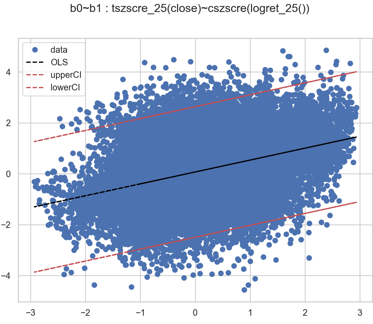
    _m3 = GeneticRegression(
        formula="tszscre_25(close) ~  cszscre(logret_25())",
        **configs
    )
    _m3_res = _m3.ols()
    print(_m3_res.summary())
    _m3.plot()
A clear positive relation as we may expect, but only in aggregate.
The decision to include momentum in the portfolio could be…well…up in the air. Speaking from data - not that relevant, but we know that markets are noisy and both effects often persist in some regimes. It could also be a reasonable diversifier. Furthermore, it could also be that the cross-sectional z-score is `rougher`, since n=10 in our study, and hence noisier than the t=25 time-series z-score.
Let us test some more artefacts/stylized facts about crypto markets. We know that volume is correlated to returns:
    m4 = GeneticRegression(
        formula="forward_1(tszscre_10(volume)) ~  tszscre_10(logret_1())",
        **configs
    )
    m4_res = m4.ols()
    print(m4_res.summary())
    m4.ols(bins=100)
    m4.plot()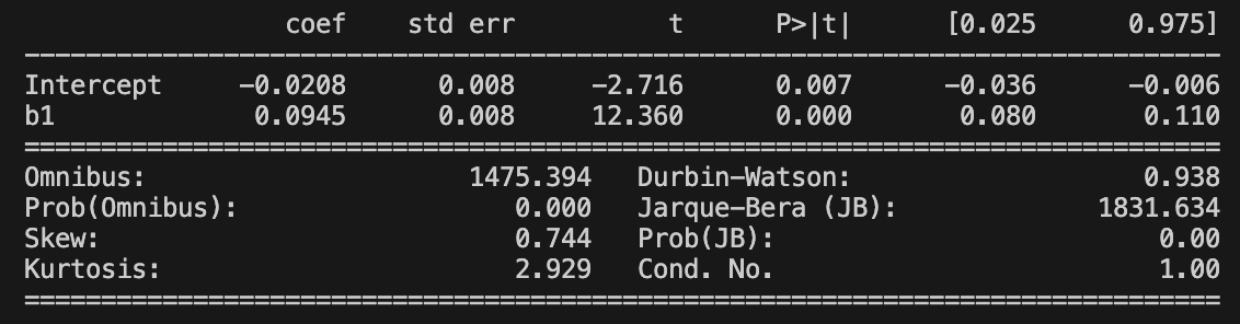
and we may be interested in smoothing variables w.r.t to volume, since statistics with large volume may be favoured over statistics generated over a thin market.
Let’s check this out:

Let’s stick to bivariate regression, those are always easier. Let’s do 3 regressions:
one-period forward return on 25-day log returns
one-period forward return on log return adjusted by volatility
one-period forward return on volume-adjusted log return adjusted by volume-adjusted volatility
    m5 = GeneticRegression(
        formula="forward_1(logret_1()) ~ logret_25()",
        **configs
    )
    m5_res = m5.ols()
    m6 = GeneticRegression(
        formula="forward_1(logret_1()) ~ div(logret_25(),volatility_25())",
        **configs
    )
    m6_res = m6.ols()
    m7 = GeneticRegression(
        formula="forward_1(logret_1()) ~ div(div(sum_25(mult(volume,logret_1())),sum_25(volume)),vwstd_25(logret_1()))",
        **configs
    )
    m7_res = m7.ols()
    print(m5_res.pvalues)
    print(m6_res.pvalues)
    print(m7_res.pvalues)
>>>
Intercept    0.008309
b1           0.000171
dtype: float64
Intercept    1.026476e-02
b1           1.161287e-07
dtype: float64
Intercept    2.352965e-02
b1           8.921023e-09
dtype: float64
they are increasingly better predictors of forward returns. It is often believed that volume is measure of entropy, and our data says possibly so.
How long does it persist?
Lets’ do just vol-adjusted returns, and see if our regression tests are in-line with the post:
    m8 = GeneticRegression(
        formula="forward_1(logret_1()) ~ div(logret_25(),volatility_25())",
        **configs
    )
    m8_res = m8.ols()
    print(m8_res.summary())
    m9 = GeneticRegression(
        formula="forward_14(logret_1()) ~ div(logret_25(),volatility_25())",
        **configs
    )
    m9_res = m9.ols()
    print(m9_res.summary())
    m10 = GeneticRegression(
        formula="forward_28(logret_1()) ~ div(logret_25(),volatility_25())",
        **configs
    )
    m10_res = m10.ols()
    print(m10_res.summary())
The regression results? Spot on (in-case you can’t download the image, the p-values are roughly 0, 0.02 and 0.7 in predicting one-day, two-week and four-week forward returns):
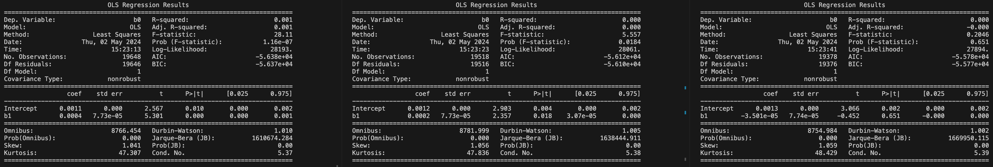
So, significance up to two weeks out.
With these regression tests, let’s run some backtests and see how they would have fared. We will run on the same tickers, same interval and data. Let’s do 5 basis points taker and 10% APR funding rate with position rollover inertia at 10%.
    strat_configs = {
        **configs,
        "instruments":tickers,
        "execrates": [0.0005] * len(tickers),
        "longswps": [0.1] * len(tickers), #annualized
        "shortswps": [-0.1] * len(tickers),
        "weekend_trading":True,
        "positional_inertia": 0.1
    }
and then let’s run a simple MAC, and MVWAP crossover, as well as the bollinger strategy. As Scott suggests, the bollinger would have done best, and as our volume regression suggests, incorporating volume might help in the signal:
    strat0 = "ite(mac_20/50(close),const_1,neg(const_1))"
    strat1 = "ite(gt(mvwap_20(),mvwap_50()),const_1,neg(const_1))"
    strat2 = "tszscre_25(close)"
    alpha0 = GeneticAlpha(genome=strat0,**strat_configs)
    alpha1 = GeneticAlpha(genome=strat1,**strat_configs)
    alpha2 = GeneticAlpha(genome=strat2,**strat_configs)
    df0 = await alpha0.run_simulation()
    df1 = await alpha1.run_simulation()
    df2 = await alpha2.run_simulation()
    plt.plot(np.log(df0.capital),label=strat0)
    plt.plot(np.log(df1.capital),label=strat1)
    plt.plot(np.log(df2.capital),label=strat2)
    plt.legend()
    plt.show()
and we get:
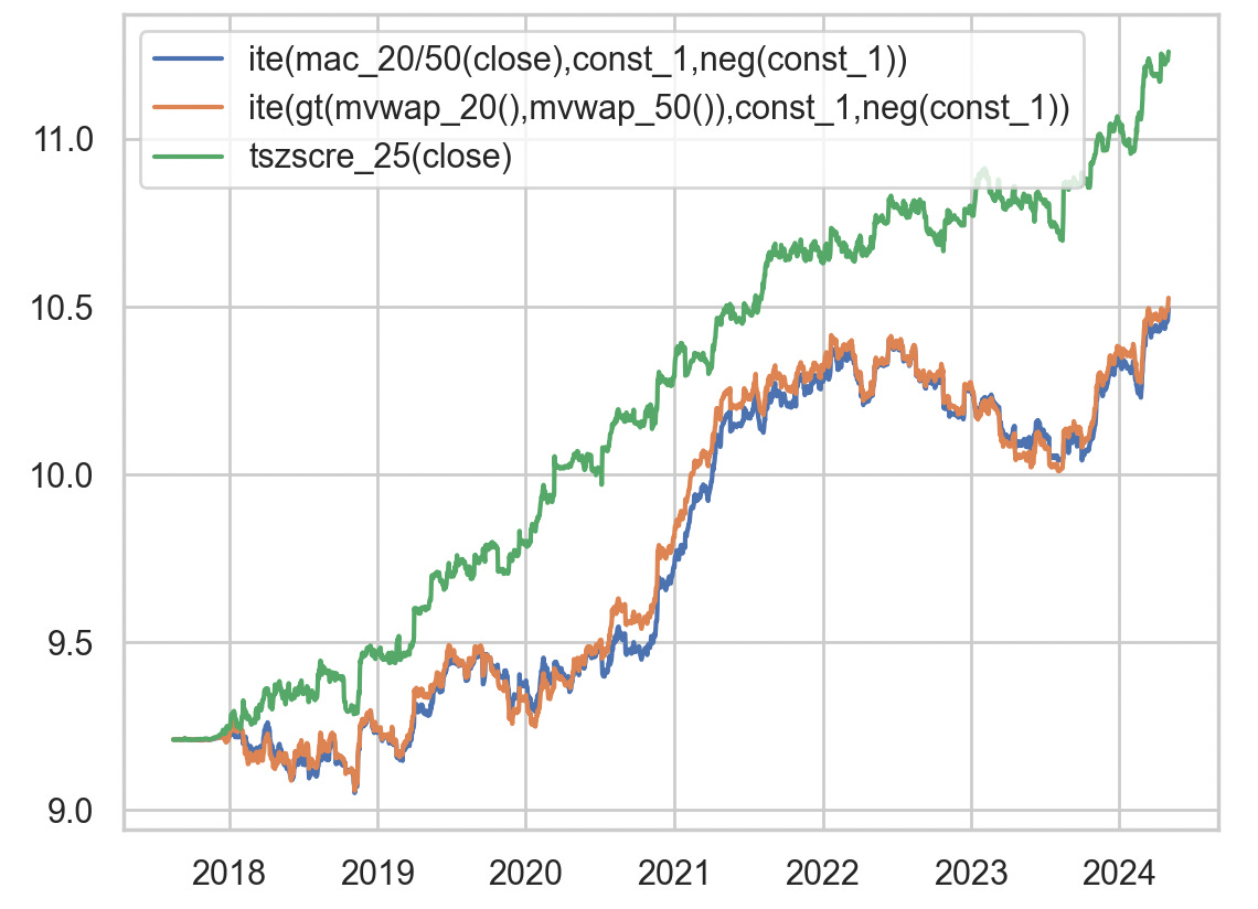
no surprise. But this might not be an apple-apple comparison, since we are comparing a digital signal to an analog one. Either way, it might be good exercise to bag and boost the crossovers to get smoother signals.
Now, let’s compare cross-sectional momentum, time-series trend and dual momentum:
    strat3 = "cszscre(logret_25())"
    strat4 = "plus(tszscre_25(close),cszscre(logret_25()))"
    alpha3 = GeneticAlpha(genome=strat3,**strat_configs)
    alpha4 = GeneticAlpha(genome=strat4 ,**strat_configs)
    df3 = await alpha3.run_simulation()
    df4 = await alpha4.run_simulation()
    plt.plot(np.log(df2.capital),label=strat2)
    plt.plot(np.log(df3.capital),label=strat3)
    plt.plot(np.log(df4.capital),label=strat4)
    plt.legend()
    plt.show()
we get:
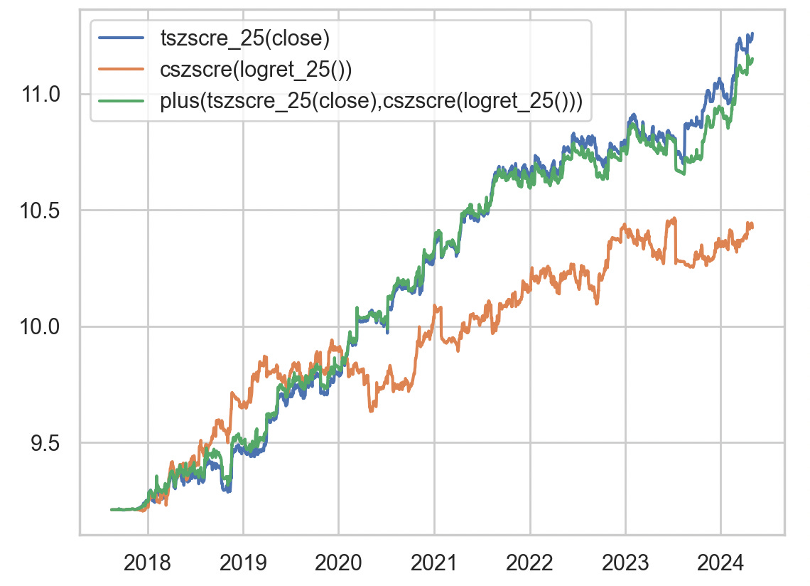
the backtests mirror our regression study. Cross-sectional momentum does well on its own, but lags behind trend-following. When combined with trend, it does not `take` much away either, and acts as an okay-diversifier. There are often periods of outperformance in one or the other.
To end off:
Trend is an edge virtually any way you do it:
    strat5 = "logret_25()"
    strat6 = "div(logret_25(),volatility_25())"
    strat7 = "div(div(sum_25(mult(volume,logret_1())),sum_25(volume)),vwstd_25(logret_1()))"
    alpha5 = GeneticAlpha(genome=strat5,**strat_configs)
    alpha6 = GeneticAlpha(genome=strat6 ,**strat_configs)
    alpha7 = GeneticAlpha(genome=strat7,**strat_configs)
    df5 = await alpha5.run_simulation()
    df6 = await alpha6.run_simulation()
    df7 = await alpha7.run_simulation()
    plt.plot(np.log(df5.capital),label=strat5)
    plt.plot(np.log(df6.capital),label=strat6)
    plt.plot(np.log(df7.capital),label=strat7)
    plt.legend()
    plt.show()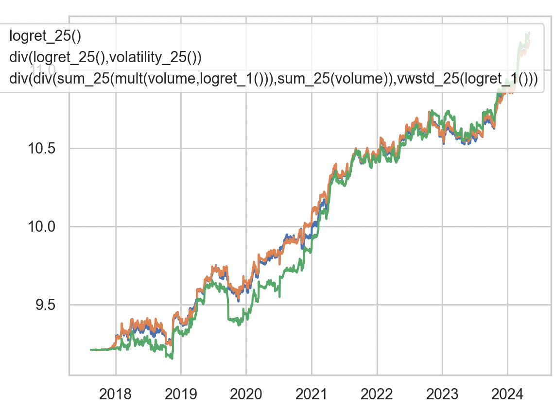
Adios~
Repo for regression and backtest: https://hangukquant.github.io/
The code (also pushed to quantpylib/dev/trend.py):